Post provided by Loke von Schmalensee
For many decades, humans have tried to understand how to process continuous signals for our convenience. As a result, numerous innovative methods have been developed for recording, compressing, restoring, and transforming (and more) continuous signals. Consider, for instance, the relationship between signal processing and music: it comes into play directly through the recording of sound waves, and indirectly via radio broadcasts. Despite the ubiquity of continuous and periodic fluctuations in nature, the seemingly vast ecological potential of signal processing theory has remained largely untapped. Here, I discuss my latest article in which I introduce two ecologically useful signal processing concepts in the context of thermal ecology. Hopefully, this blog post provides an alternative angle, focusing on conveying the intuition for why these signal processing concepts work.
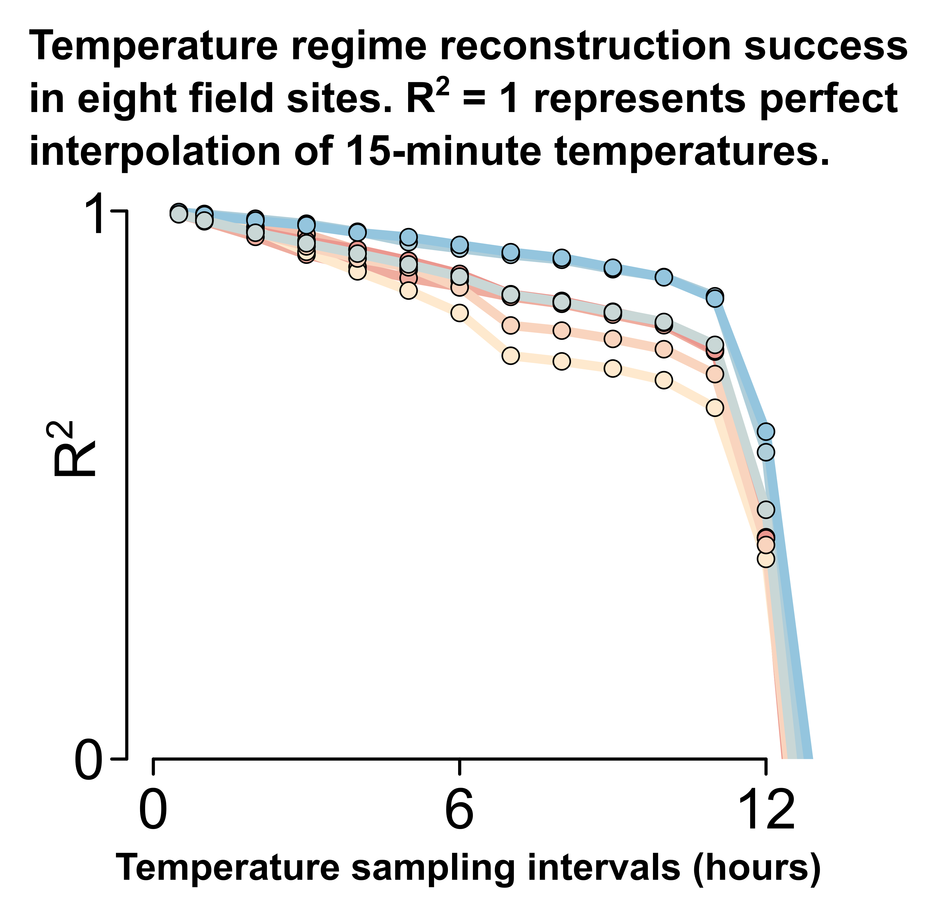
I had just presented the first chapter of my PhD dissertation (at the time of writing, I am still a PhD student) when my friend who attended the presentation, Klas Walldén, approached me. He pointed out that one of our findings (namely, that increased frequency of microclimate measurements only improved predictions of insect development times when measurement intervals were 12 hours or shorter) reminded him of a concept he had encountered while studying engineering physics—the “Nyquist-Shannon sampling theorem“. Although intrigued, I did not give it much thought at the time, as I was preoccupied with other ideas. A year later, Klas’ comment resurfaced in my memory, prompting further exploration. I learned that, under the right conditions, continuous signals could be reconstructed from surprisingly (at least to me) infrequent measurements, and I realised that these interpolation techniques could be applied to my microclimate temperature datasets to increase their temporal resolution. Eventually, this resulted in an article about the applicability of the Nyquist–Shannon sampling theorem and sinc interpolation in thermal ecology. Here, I describe the article’s content from a slightly different perspective, sharing the intuitions I have gained in a way that is hopefully accessible to fellow ecologists. But to summarize the main result: most natural temperature variation in time-series of measurements taken every 15 minutes (i.e. temporally high-resolved data) could consistently be retrieved when temperatures were sampled only every 11 hours (see figure below).
Getting around the math stuff
The foundational references in my article (e.g., Shannon 1948) are quite packed with mathematical notation. As an ecologist, I do not appreciate mathematical notation as much as I do math. As with musical scores—I can read it in theory, but it will likely take longer than the author intended. In other words, mathematical notation is an inefficient way of communicating mathematical ideas to me, and I suspect I am not alone in this among ecologists. Perhaps, favouring mathematical notation over figures and plain text might even create barriers for ecologist readers, leading them to overlook relevant and important findings (which, ironically, might be the reason I could write the article). Therefore, I here use precisely plain text and figures to elucidate some concepts underlying my article, with the aim of making them more accessible. As a trade-off, I must apologise in advance to the meticulous mathematician or engineer for the crudeness of my explanations.
The power of Fourier series
A key player in this story is the mathematician Jean-Baptiste Joseph Fourier and his discovery of Fourier series (coincidentally, he made the discovery while working on heat conduction). Fourier proposed that mathematical functions could be represented as infinite sets of sinusoids (i.e. sine and cosine waves), or “Fourier series”. Granted, another mathematician with an equally lengthy name, Johann Peter Gustav Lejeune Dirichlet, later showed that certain conditions need to be satisfied for this to be true. Nevertheless, a remarkable range of functions can at least locally be well-approximated by simply summing sinusoids, emphasising the significance of Fourier’s discovery. From this, it is reasonable to assume that temperature regimes too can be approximated by summing sine and cosine waves. This is indeed the case, as demonstrated in the figure below.
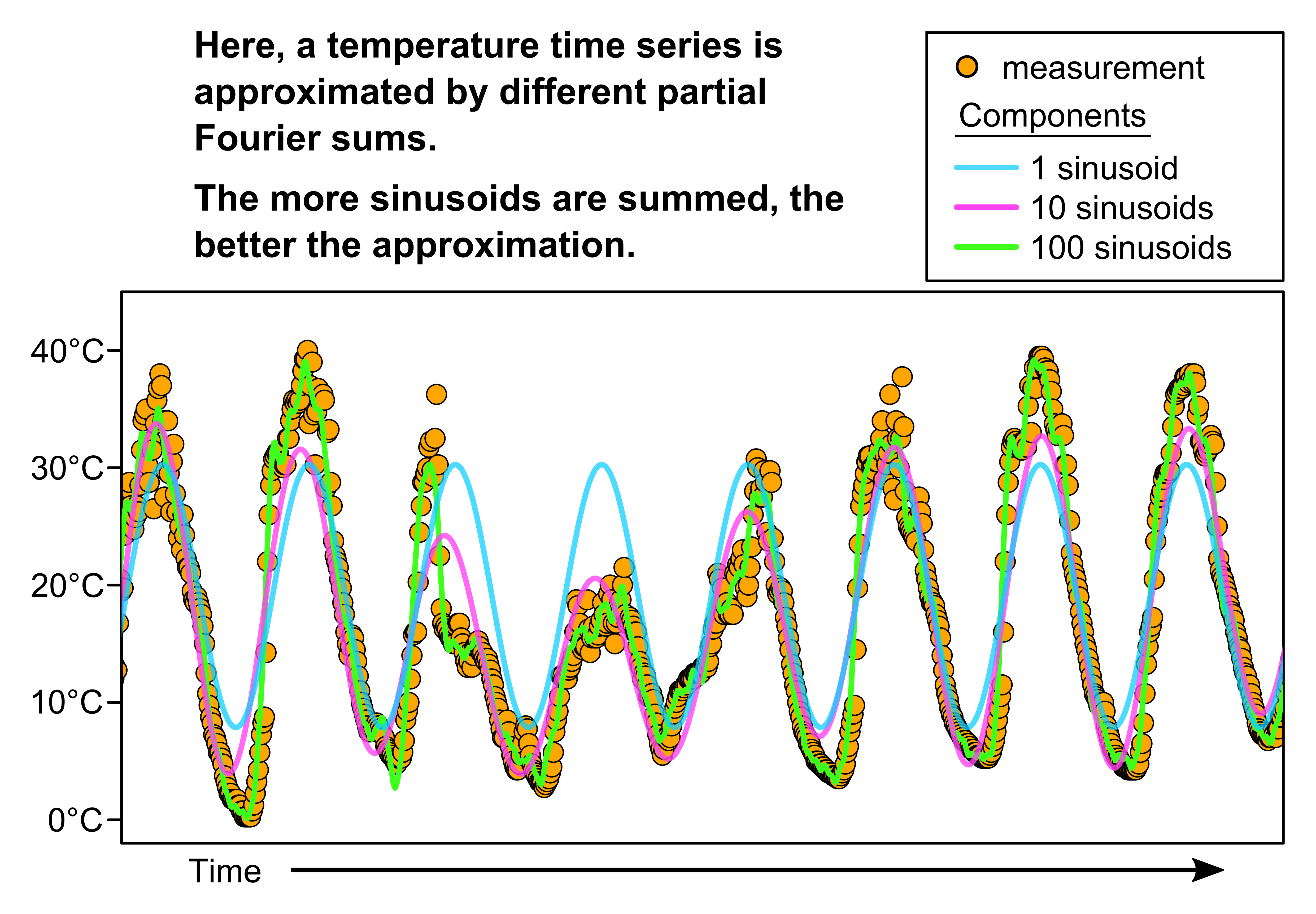
As will become evident, this simple fact—that temperature regimes can be broken down into separate sinusoids (a.k.a. frequency components)—is fundamental for my article’s application of signal processing theory.
Why can signals be reconstructed?
In my article, I introduce the Nyquist–Shannon sampling theorem, which states that frequent enough sampling allows continuous signals to be perfectly reconstructed from discrete measurements (through “sinc interpolation” in the time domain, or “zero padding” in the frequency domain). I will not write about the interpolation techniques here (for that, please see the article). Instead, I will attempt to convey my intuition for why a continuous signal can be perfectly reconstructed from discrete measurements by exploring a simple example: a single sine wave.
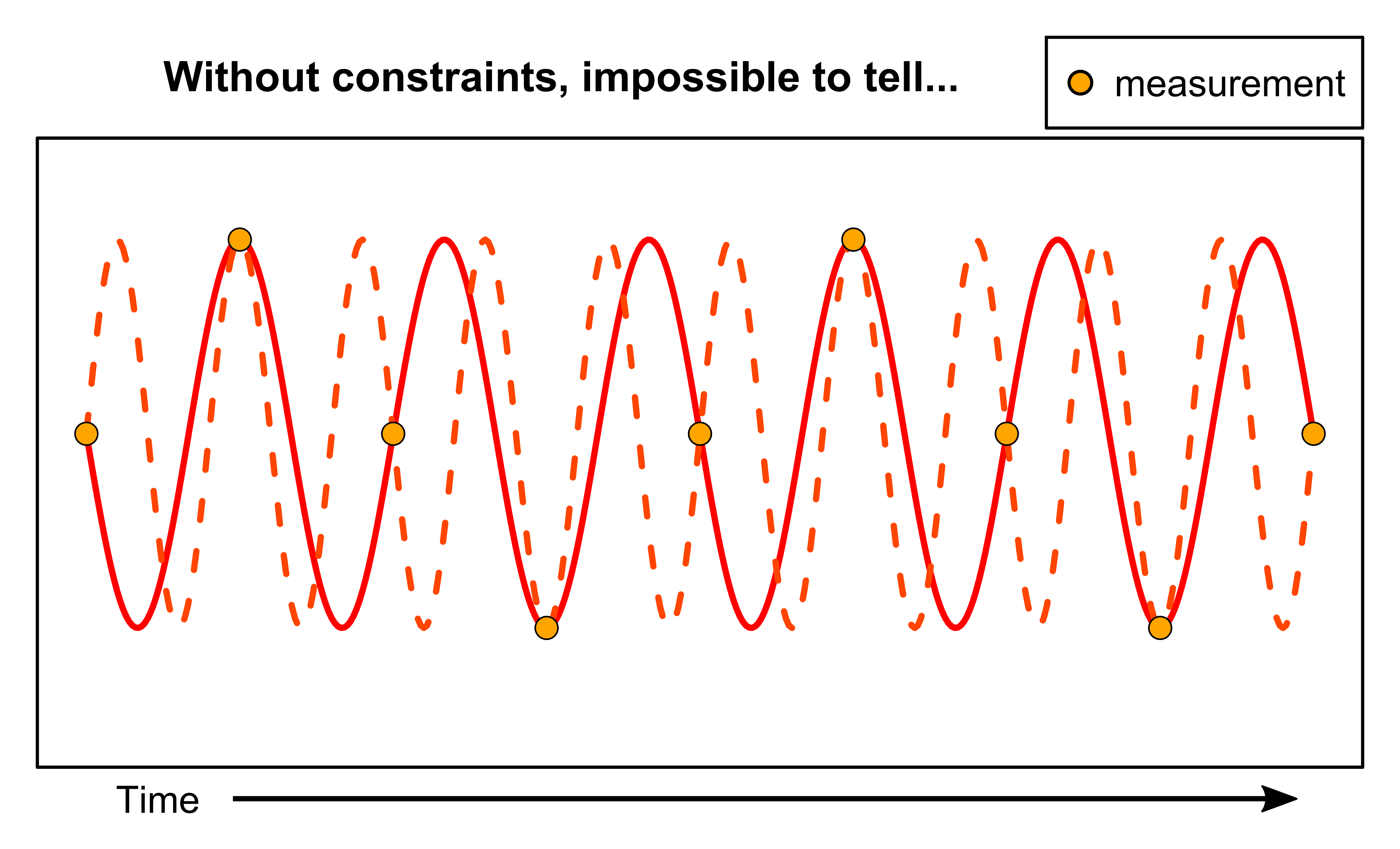
Imagine wanting to reconstruct an unknown sine wave within a time series consisting of evenly spaced measurements. You begin by visualising the measurements (below).

What could possibly be the true wavelength of that signal? Perhaps, you connect the dots in time and see a triangle wave appearing. You might think to yourself: “A-ha, a sine wave with the similar characteristics as this triangle wave would also fit the data. That must be the solution!” But that would be ill-advised. Without imposing any constraints on the frequency of the sine wave you are looking for, there is no way for you to find a solution. In fact, given these measurement time points, there is an infinite number of frequencies that would generate the same data. See the figure below for two examples.
The Nyquist-Shannon sampling theorem says that perfect reconstruction of a sinusoid can be achieved when (periodic) sampling happens at least twice every wavelength. In other words, the interpolation algorithms operate under the assumption that no frequency components in the sampled signal have wavelengths shorter than twice the sampling interval (note: in contrast to the example of the single sine wave used here, a signal can be a complex waveform expressible as the sum of a set of sinusoids). Under this assumption there exists a unique solution to our question, as demonstrated in the figure below (the black line represents this unique solution; the pink lines represent the signals in the previous figure).

In this figure, it is also apparent that not measuring the signal frequently enough can lead to substantial errors. Imagine if the true signal was actually the solid pink line, not the black one. The pink signal would result in the exact same measurements as the black signal when taken at the particular time points used here (as shown by the orange points). Consequently, even when the true signal is actually the pink solid line, the measurements intervals used here will produce the black signal in a waveform reconstruction. This phenomenon is known as aliasing: if the signal is under-sampled according to the Nyquist–Shannon sampling theorem, high-frequency waves are interpreted as lower-frequency waves. Hence, aliasing can cause varying grades of distortion in the reconstructed signal depending on the relative amplitude of the under-sampled high-frequency component.
It follows from this that for a signal to be perfectly reconstructed from discrete samples, it must only contain frequency components within a limited frequency range; to capture a wave with an infinitely high frequency requires infinitesimal measurement intervals, so the frequency spectrum must be bounded at some high frequency. A signal with such a bound on its frequency content is called “band-limited”.
(The term “band-limited” has remained somewhat confusing to me. When I studied music production, I learned that a “band-pass filter” would explicitly filter both upper and lower frequencies. However, since physical frequencies cannot be negative, I guess that one could say that even a just an upper frequency cut-off—a low pass filter—results in a band-limited signal, since the signals frequency content necessarily is bounded at zero.)
Why signals can be reconstructed
We have now identified some important criteria upon which the Nyquist–Shannon sampling theorem relies: (1) the signal is sampled at even time intervals, (2) the signal can be broken down into separate sinusoids (there is our connection to the Fourier series!), and (3) the signal is band-limited. Under these conditions, a continuous signal can be perfectly reconstructed from discrete measurements (the assumption of infinite time series which can be ignored for most ecological purposes). However, according to the Nyquist–Shannon sampling theorem, this can generally only be done if the signal is measured at a rate at least twice that of its highest frequency component. But if the sampling rate is sufficient and the other conditions are met, there exists just a single solution to the problem of fitting a complex sinusoid to a time series of measurements—the true signal!
What about temperature regimes?
In reality, band-limited and noise-free signals are hard to come by. Thus, aliasing will happen, and there exists a whole range of ingenious techniques designed to reduce aliasing in under-sampled signals. However, frequency spectra of temperature time series are generally defined by negative relationships between amplitude and frequency, meaning that rapid fluctuations contribute relatively little to the total temperature variation (see also the article and references therein). Therefore, failing to capture these rapid fluctuations might not lead to significant distortion.
In conclusion, relatively low-resolved temperature time series can capture the most significant frequencies at which temperatures fluctuate. At the same time, more rapid fluctuations that are not captured by the sampling causes relatively little distortion (through aliasing) in the reconstructed temperature regime because of their low amplitudes. This is why continuous temperature regimes can be efficiently reconstructed from temporally sparse temperature data. Why does this matter, ecologically? Well, for ecological models, summary statistics of environmental temperature distributions simply do not cut it—temperature changes generally have different biological meaning depending over what temperatures they occur. Therefore, the ability to generate continuous temperature regimes will aid ecologists in creating meaningful models of temperature dependent responses in nature.
