
Post provided by Maëlis Kervellec
An Increased Interest Towards Landscape Connectivity
Human activities not only contribute to climate change by producing greenhouse gases, but also directly degrade habitats. According to the 2019 IPBES report , about 75% of the Earth’s land surfaces have been heavily modified. Moreover, in Europe, 50% of the land is within 1.5 kilometres of a road (Torres, Jaeger, and Alonso, 2016 ). This fragmentation of landscapes is a major concern. It makes it harder for animals to move, whether for daily needs like finding food or to recolonise areas from where they were extirpated. This leads to smaller, isolated populations, less genetic diversity, and ultimately a decrease in species richness.
To address these challenges, the concept of landscape connectivity has gained a lot of attention from scientists to politicians. This term describes how easy it is to move across a landscape. It has become a key idea in conservation plans globally. In 2022, countries around the world adopted the Kunming-Montreal Global Biodiversity Framework (GBF). Out of 23 targets set for 2030, five focus specifically on improving connectivity between habitats to stop biodiversity loss.
Growing Focus in Landscape Ecology
Despite the global agreement to reduce habitat fragmentation, figuring out how to measure and improve connectivity isn’t easy. The science of connectivity has grown rapidly to provide tools for understanding how landscape features affect animal movement (for more information, check out https://conservationcorridor.org). However, many current methods fail to propagate the uncertainty from the data to the connectivity maps .
Addressing uncertainty in ecological studies
Hierarchical models help solve this problem. These models can separate the observation process from the actual ecological process. For example, just because a species wasn’t spotted at a specific location doesn’t mean it wasn’t there. Many factors, such as weather or the experience of the person doing the survey, can influence whether a species is detected. In our research, we used occupancy models, which rely on detection and non-detection data collected from sites surveyed multiple times per year. The observation process deals with the variability in detectability, while the ecological process, in our case, focuses on what factors impact the distribution of a species.
Traditionally, models explaining species distribution made simple correlations between habitat features (like forest cover or distance to human settlements) and the presence of species. However, the closer two locations are, the more likely this localisation is also occupied by the species. Methodological developments included this “as-the-crow-flies” distance, called Euclidean distance, to account for the spatial structure in species distribution.
Ecological Distances: Going Beyond Straight Lines
But landscapes are rarely simple and open. There are barriers like rivers or highways, and corridors like forest patches that make movement easier. This is where developments in landscape ecology come in. Ecological distances take into account these landscape features to show how close or far apart two locations really are. For example, imagine you need to buy pastries. Will you choose the bakery right in front of your house but across a river, or the one near the bus stop on your way to work?
In 2018, Paige Howell and colleagues , used an ecological distance called the least-cost path distance into a species distribution model (called occupancy model) to study frog recolonisation while accounting for the cost of elevation on their movement. This distance assumes that animals will take the easiest, most direct route. However, this distance doesn’t consider the presence of multiple routes to a location, which can make it more accessible. Going back to the bakery example, imagine that your favourite bakery can only be reached by a single bus line, while another is connected by several. Most people would likely choose the second one because it offers more convenient ways to get there.

 estimated by the model and a spatial covariate, here the presence of the road. The proximity between the four occupancy sites (blue points) is defined according to the commute-time distance. This distance is computed between all pairs of orange nodes that match the centre of the occupancy sites. Note that the resistance surface has a larger extent and a finest resolution than the occupancy surface to allow multiple routes between sites. The focal species can be present (denoted 1) or not (denoted 0) at each occupancy site (in blue). Occupancy state at each site in the following primary occasions arises from a site colonisation probability (
 and the commute-time distance to occupied sites in the previous primary occasion. At each site, we conducted in this example three repeated secondary occasions where the focal species can be detected (1) or not (0) and is presented here on the detection surface (in yellow).
A New Approach: Using commute-time distance in species distribution models
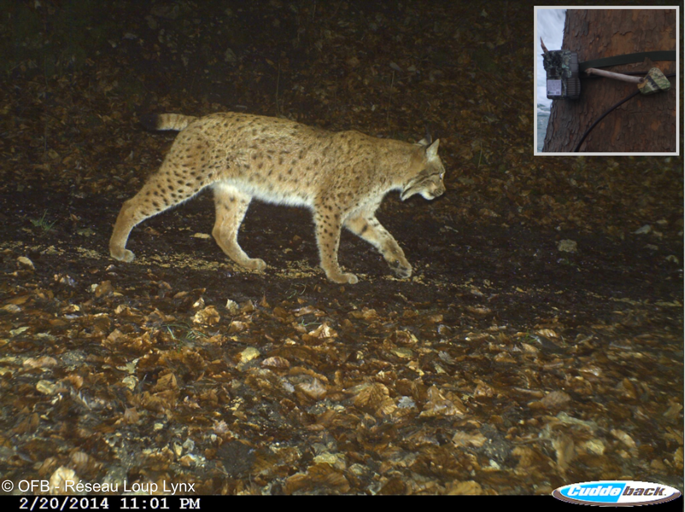
In our research, we replaced the least-cost path distance with commute-time distance from circuit theory. This method considers all possible routes between locations, not just the most efficient one, to better represent accessibility, much like several bus lines connecting the same destination. We applied this model to two species recolonising highly structured landscapes in France: The Eurasian lynx and the Eurasian otter. Our findings showed that rivers facilitated the otter’s recolonisation, while highways acted as barriers, limiting the lynx’s movement.
A unifying tool for population conservation
Landscape ecology offers many approaches that more accurately reflect how species move through fragmented environments. By integrating these models with hierarchical approaches, we create a powerful tool that not only captures species movement but also accounts for uncertainties in the data. Bridging the gap between landscape ecology and hierarchical models opens up new possibilities for more realistic and precise predictions of species distribution. It allows us to incorporate any ecological distance that aligns with a species’ movement patterns. Strengthening this link will help us better understand landscape connectivity and make more informed conservation decisions.
You can read the full article here.
Post edited by Sthandiwe Nomthandazo Kanyile
