Post provided by JENNY HODGSON
Climate change and habitat fragmentation are interacting threats: it is likely that many species cannot reach newly suitable areas at the cool edge of their range because there is not enough habitat, in the right places, to support range expansion over multiple generations. Conservation efforts are already underway to restore large areas of habitat, and to improve the “connectivity” within networks of habitat. However, there are multiple ways of measuring connectivity and few of them address the scale of shifts that are likely to be needed under climate change. This could be a problem if it leads to inefficient conservation prioritisation.
The Conductance Metric
We first developed the conductance metric in 2012 and we found that it is correlated to the speed with which a species can spread through a landscape, from a specified source location to a specified target. A key difference between this and most other connectivity metrics is that it incorporates both reproduction within habitat patches and dispersal between habitat patches, over multiple generations (further explanation here). Sometimes there could be many very well-connected patches in a network, and yet no easy way for a species to cross the landscape from end to end. This could be a problem for the species’ survival, if staying within its current regions of occupancy is unsustainable, for example if it is being pushed northwards by climate change.
Our latest work investigates how one could gradually modify an existing landscape in order to optimise its conductance between a fixed source and target. If we can compute optimal arrangements quickly, given knowledge about the existing habitat and the land available for conservation or restoration, this could be an important ingredient in building decision support tools. For the moment though, we’re demonstrating our methods in simplified scenarios: in particular, we are assuming that the conductance for one species in one direction (south-north) is the only conservation goal for the landscape.
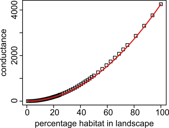
First, we investigated how conductance depends on the total area of habitat in the landscape. It may seem obvious that conductance increases with more habitat, but showing how it increases is still interesting and useful. When habitat cells are added to a raster landscape at random, the conductance increases in proportion to the amount of habitat squared (see figure above). One implication of this for everyone is that habitat restoration can have benefits even when nothing is known about how to optimise the arrangement: adding habitat completely at random still helps. We also needed this information to prove that our new methods are much better than random at choosing which habitat patches to add or retain.
Optimising Restoration of Habitat Networks
There are two broad approaches people may take towards prioritising or optimising the restoration of habitat networks. They may wish to pinpoint the absolute best place to add a habitat patch to the existing network or they may have a restricted map of possible restoration patches that they wish to choose between. So, we developed an “adding” routine for the first approach, and a “dropping” routine for the second approach.
In the dropping routine, we repeatedly calculate which patch is contributing least to the overall conductance, then delete this patch and recalculate. This may seem like the opposite of what a conservationist wants to do, but if we can thin down the network and show that conductance remains as high, or nearly as high as it started, this is very good way of showing the high importance of the patches that are retained. It’s important to note that this doesn’t imply that the other patches should literally be deleted from the landscape.
Our dropping routine uses the metric of “patch flow” to decide which patch to drop. Consistently across 30 test landscapes, we could drop 25% of cells without losing more than 6% of the starting conductance. The figures below show the relative flow attributed to patches before dropping started, and then the order in which 50% of the patches were dropped.

Our adding routine examines the links in the habitat network – which are constructed based on the probabilities of colonisation from one patch to another – and finds the link with the highest “power”. High-power links turn out to be places where resistance in the circuit is causing a problem for the overall conductance. Our routine reduces the resistance by placing one additional habitat patch at the midpoint of the link with the highest power, and then recalculates both the conductance and the power. After adding 24 cells with this routine to 30 test landscapes that started with 1024 cells, we increased conductance by a minimum of 24% and a median of 3,800%. The expectation based on adding habitat at random would be a 4.7% improvement. The spatial patterns created by this routine makes sense as chains of stepping stones spanning the most significant gaps between the north and south edges of the landscape (see the figure below).

The Next Steps
We are excited by these methods because they start to bridge the gap between methods for visualising connectivity pathways, which do not offer straightforward suggestions for improvement, (except McRae et al) and true conservation optimisation tools such as ZONATION and Marxan, which only incorporate very simple connectivity measures.
Some of the methods developed in this paper are already implemented in our desktop software Condatis version 0.6.0. But if you want to check out the adding routine you’ll have to wait for the next version or look at the R code in the supplementary material.
The next steps in this research will be to think about optimising for multiple species in multiple directions, and about prioritising for long-term survival in one place as well as the speed of range shifting. If you are thinking about using, testing, or building on these methods we would love to hear from you (jenny.hodgson[at]liverpool.ac.uk).
To find out more about the conductance metric, read our Methods in Ecology and Evolution article ‘How to manipulate landscapes to improve the potential for range expansion’.

2 thoughts on “Planning Habitat for Very Long-Distance Connectivity under Climate Change”