Post provided by Cornelia Oedekoven
The Standard Method
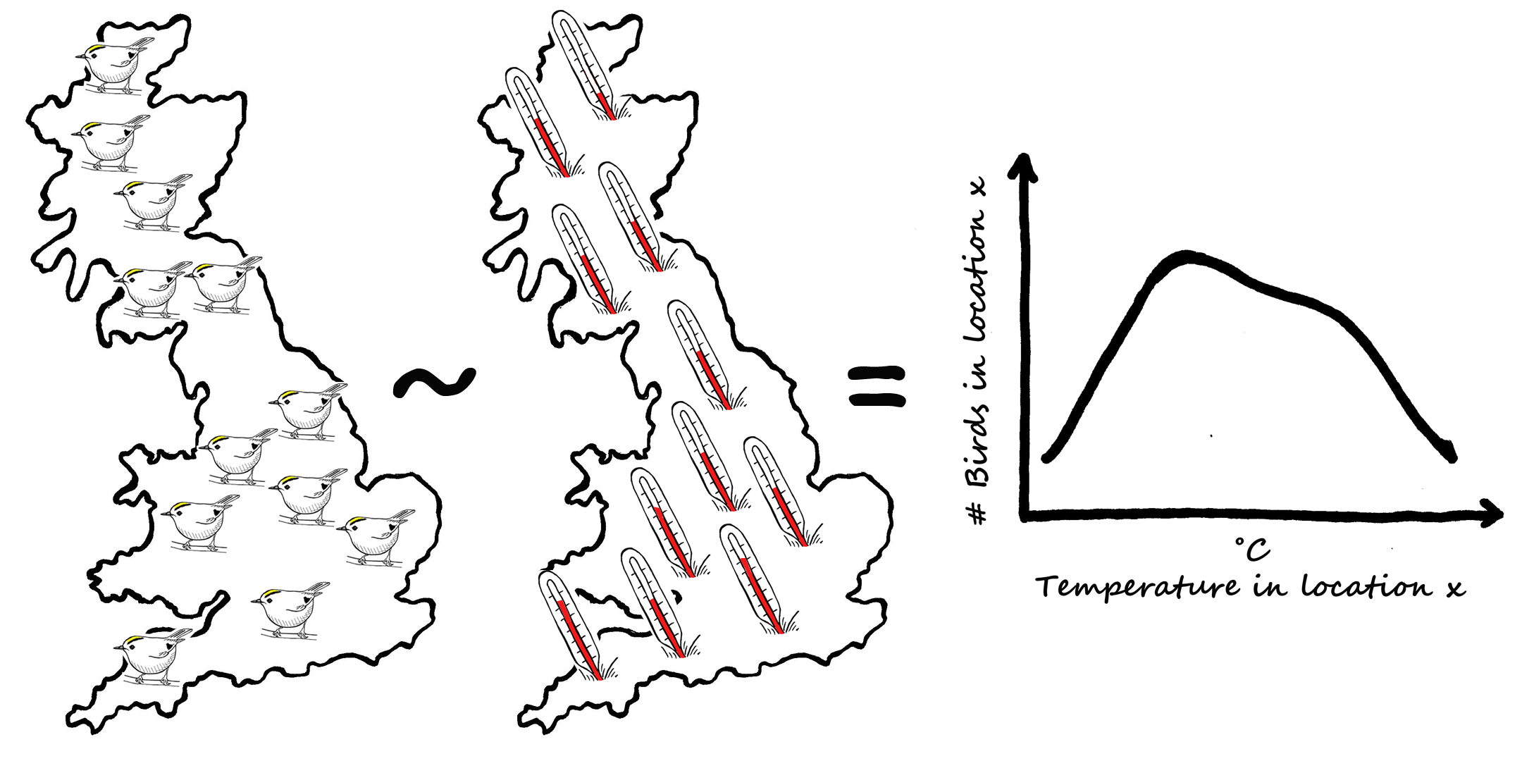
When trying to understand how wildlife, for example a bird species, may react to climate change scientists generally study how species numbers vary in relation to climatic or weather variables (e.g. Renwick et al. 2012, Johnston et al. 2013). The way this tends to be done is by gathering information (data!) about bird numbers as well as the weather variables (for example temperature) in several locations (i.e. in space) and fitting a regression model to these data to detect and illustrate how bird numbers go up or down with temperature.
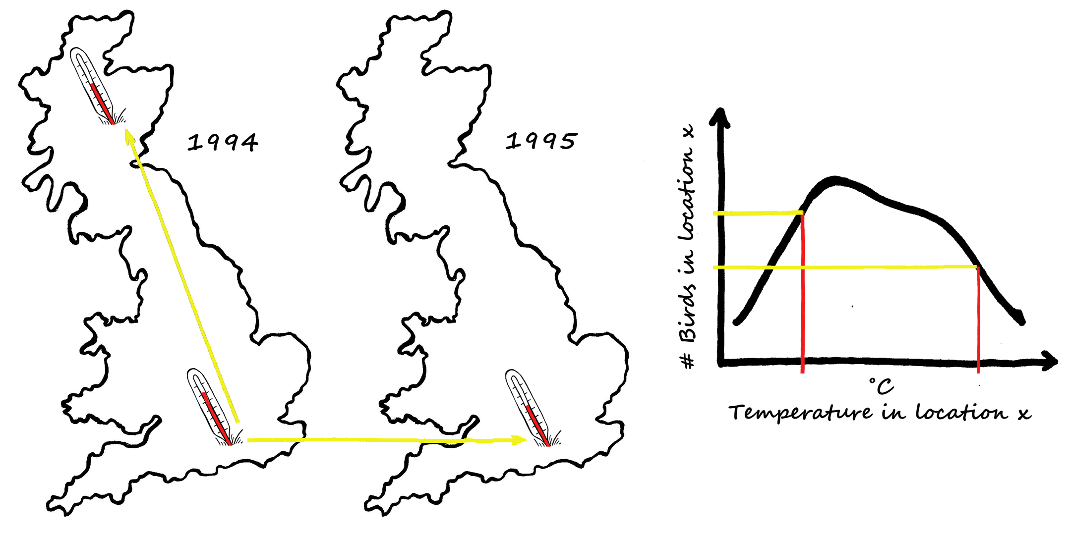
This relationship is then used to forecast how bird numbers may change along with potential temperature changes in the future (i.e. in time), for example due to climate change.

Confounding Issues?
There is potentially a confounding issue in the standard method though. Using this method means that, for example, we would have to believe that a change in temperature in one location from 12°C to 13°C (temporal variation) would have the same effect as the difference between two locations at one point in time (spatial variation), one location at 12°C and one at 13°C. In technical terms: the standard method confounds the spatial and temporal effects of the weather variable on bird numbers.
One of the potential reasons the standard method may be confounding is local adaptation (i.e. that birds are adapted to local average temperatures). For example, individuals of the same species that live in locations where temperatures are colder on average may perceive 20˚C as too hot, but individuals living in places with warmer average temperatures may wish it was a bit warmer. (Similar to how some Scottish folks might complain about the heat when temperatures rise to 20˚C on a summer day while English folks may be happy if temperatures rose a bit more).

What’s New about Our Methods?
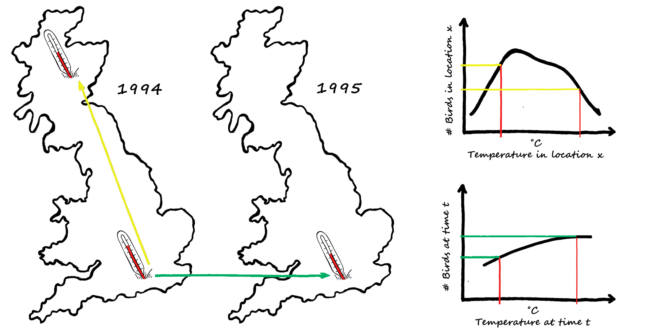
We developed a new approach to distinguish between temporal and spatial variability in any particular weather variable. Our methods allow the relationship between bird numbers and temperature (or any wildlife species and climate variable in general) to differ spatially and temporally.

How does it Work?
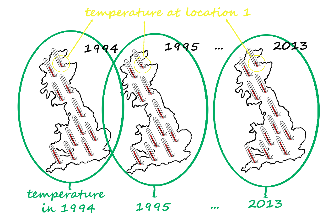
First, we need data on bird numbers and temperature on a good spatial and temporal resolution (i.e. bird count and temperature measurements from lots of locations and lots of time points).

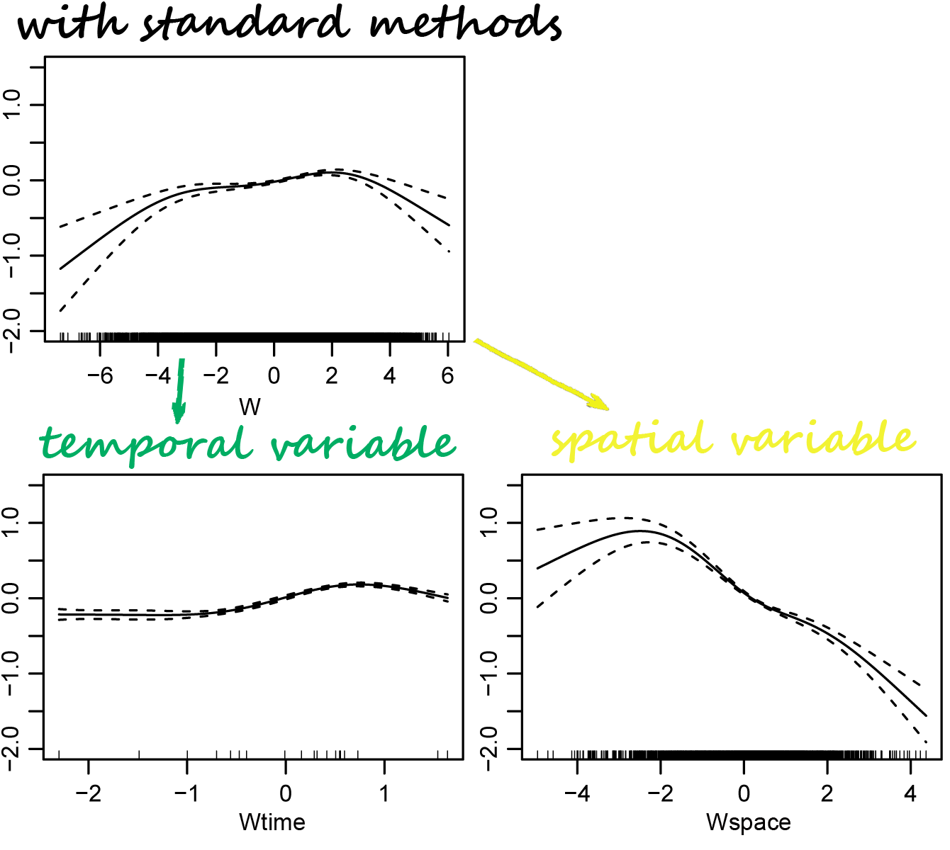
We split up the weather variable into new variables by separating out temporal and spatial variation in temperature (and actually a third variable, the residual variation which you can read about in our paper). We then relate bird numbers to these new variables.
Citizen Science Data Hard at Work!
 We illustrate our new approach using bird counts from the UK’s Breeding Bird Survey (BBS), a large-scale biodiversity monitoring program coordinated by the British Trust for Ornithology (BTO). Sampling sites for the BBS are randomly selected 1km squares throughout Britain (~1500 in 1994 increasing to 3350 in 2013). During the survey, volunteers walk two parallel 1km transect lines following a distance sampling protocol where they assign each bird that they detect to one of four distance categories (0-25m from the transect line, 25-100m, >100m, flying).

Weather Data from the UK Government Met Office
 We used three weather variables from the Met Office: minimum temperatures during the winter and mean temperatures and rainfall during the preceding breeding season which we obtained. We also used elevation and land class variables for our analyses as other studies have shown that they affect bird distributions in the UK.
What did We Find?
We were able to establish better relationships between bird numbers and weather variables by using our new methods for each of the five bird species. Check out how the relationship between goldcrest numbers and minimum winter temperatures changed when we divided it up into the spatial and temporal covariates.
Model Predictions and Distribution Maps
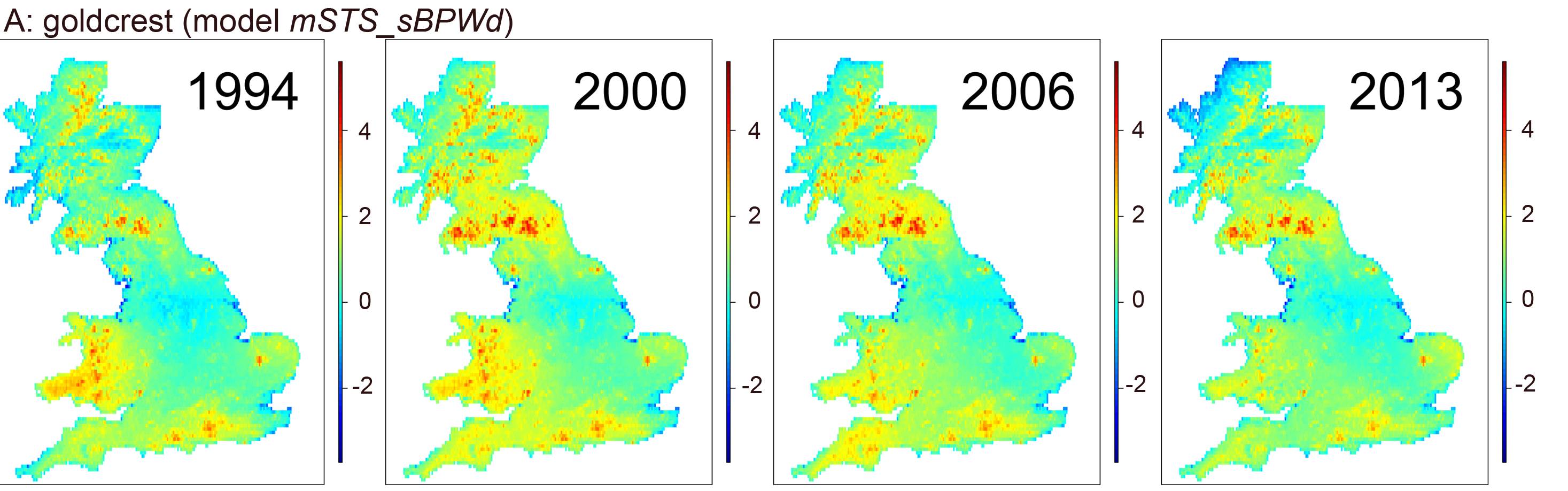
We can use the established relationships to estimate how many birds we expect to find in any location in Britain. The figure below from our paper shows the estimates for goldcrest for four selected years, illustrating how abundances fluctuated between years and in different locations. Note the decrease in abundances of goldcrest throughout Scotland and Wales in 2013 compared to previous years.
What do We Conclude?
Spatial variation in climate may affect the long-term equilibrium of species abundances by impacting the average habitat, food resources and indirectly the biotic competition. Temporal variation in weather may be more likely to have immediate effects, such as changing survival or productivity, through physiology, food availability, or breeding conditions (e.g. Robinson, Baillie & Crick 2007, Pearce-Higgins et al. 2015). Our proposed methods have the potential to assist in disentangling these multiple processes in a single analysis.
What Have We Achieved?
Our methods estimate the effect of temporal changes in weather, while accounting for spatial effects of long-term climate. This improves inference on overall and/or localised effects of climate change. With increasing availability of large-scale data sets, the need for appropriate analytical tools is growing. Our proposed decomposition of the weather variables represents an important advance by eliminating the confounding issue often inherent in large-scale data sets.
What Next?
Given the multi-dimensional nature of climate change, developing tools for incorporating multiple climatic factors will ultimately be required to more fully model the overall impact of climate change on species’ populations. The general increase in well-designed species recording schemes will provide a greater range of response variables; the expansion of land-based and aerial earth observation has potential to provide covariate data with fine temporal and spatial resolution. So, it is reasonable to expect that our methods will become more and more applicable in future.
To find out more read our Methods in Ecology and Evolution article ‘Attributing changes in the distribution of species abundance to weather variables using the example of British breeding birds’.

Wonderful explanation – thank you!