Post provided by Gurutzeta Guillera-Arroita

Species Surveys: New Opportunities and Ongoing Data Challenges

Monitoring is a fundamental step in the management of any species. The collection and careful analysis of species data allows us to make informed decisions about management priorities and to critically evaluate our actions. There are many aspects of a natural system that we can measure and, when it comes to monitoring the status of species, occurrence is a commonly used metric.

Ecologists have a long history of collecting species occurrence data from systematic surveys and our ability to gather species data is only going to grow! This is partly enabled by the fact that citizen science programs are starting to gain a prominent role in wildlife monitoring. There’s a growing recognition that well-managed citizen science surveys can produce useful data, while scaling up monitoring effort thanks to the increased human-power from large numbers of committed volunteers.

The advent of new technologies is also enhancing our monitoring abilities. New approaches to data collection continue to emerge: drones, thermal sensors and acoustic loggers are a few examples of how technological developments are opening up a wealth of new opportunities for wildlife monitoring.

While all of these developments are exciting, we must remember that most survey methods are imperfect. There are two ways in which species occurrence records can be mistaken:

• False negatives – We may wrongly record a species that is present at the site as “absent”. This is the most prevalent error in wildlife surveys. (It’s often an issue even in surveys of sessile species!) With realistic survey effort, it is usually unlikely for detection of species to be 100% guaranteed.
• False positives – On the other hand, we may wrongly record a species as present at a site where it does not occur, perhaps because it is mistaken for a similar species. Methods that rely on indirect observation of species are more likely to run into this sort of problem. It has, for instance, been shown that false positives can be widespread in aural bird surveys.

Accounting for Imperfect Detection: Ambiguity about Parameter Values Requires Data Integration

The good news is that we can deal with both of these error types in the estimation of occurrence probabilities. We do this by taking a hierarchical approach to modelling, where the state and observation processes are described separately (see a review of these methodologies here). This does not come for free though. Fitting such models requires having suitable data that can tell us about the probabilities with which false negatives and/or false positives are generated: it is not enough with a single “presence/absence” record per site.

A common way to account for false negatives is to conduct repeated visits to survey sites. These data let us estimate the probability of species detection at sites where it is present.  Survey protocols like this and corresponding data analyses are widely applied in ecology – they’re often simply referred to as “occupancy modelling”.

Things become a bit more complicated when false positives are also a potential issue. Unless some additional information is brought in, fitting a model that allows for false positive and false negative errors will yield ambiguous parameter estimates. Imagine a system where the species occupies 30% of the sites (occupancy psi=0.3), and a monitoring method that detects the species in 70% of surveys at sites where it is present (true detection probability p₁₁=0.7) and falsely records it in 10% of surveys at sites where it is absent (probability of false positive p₁₀=0.1). It can be shown mathematically that, regardless of the amount of replicated detection/non-detection data we collect, our analysis will not be able to distinguish whether the values of the parameters are {psi=0.3, p₁₁=0.7, p₁₀=0.1} or whether they are {psi=0.7, p₁₁=0.1, p₁₀=0.7}. A number of approaches have been proposed to resolve this ambiguity. These include augmenting the dataset with records from an unambiguous detection method at some sites, classifying detections according to whether they are certain or uncertain, confirming a subset of detections after data collection (e.g. DNA testing on scats), or running calibration experiments that directly inform about error rates.

[A note of caution here: while all these modelling developments are great, you should aim to minimize data collection errors in the first place, rather than waiting to “fix” things at the modelling stage.]

Environmental DNA Surveys: Potential Detection Errors at Multiple Levels

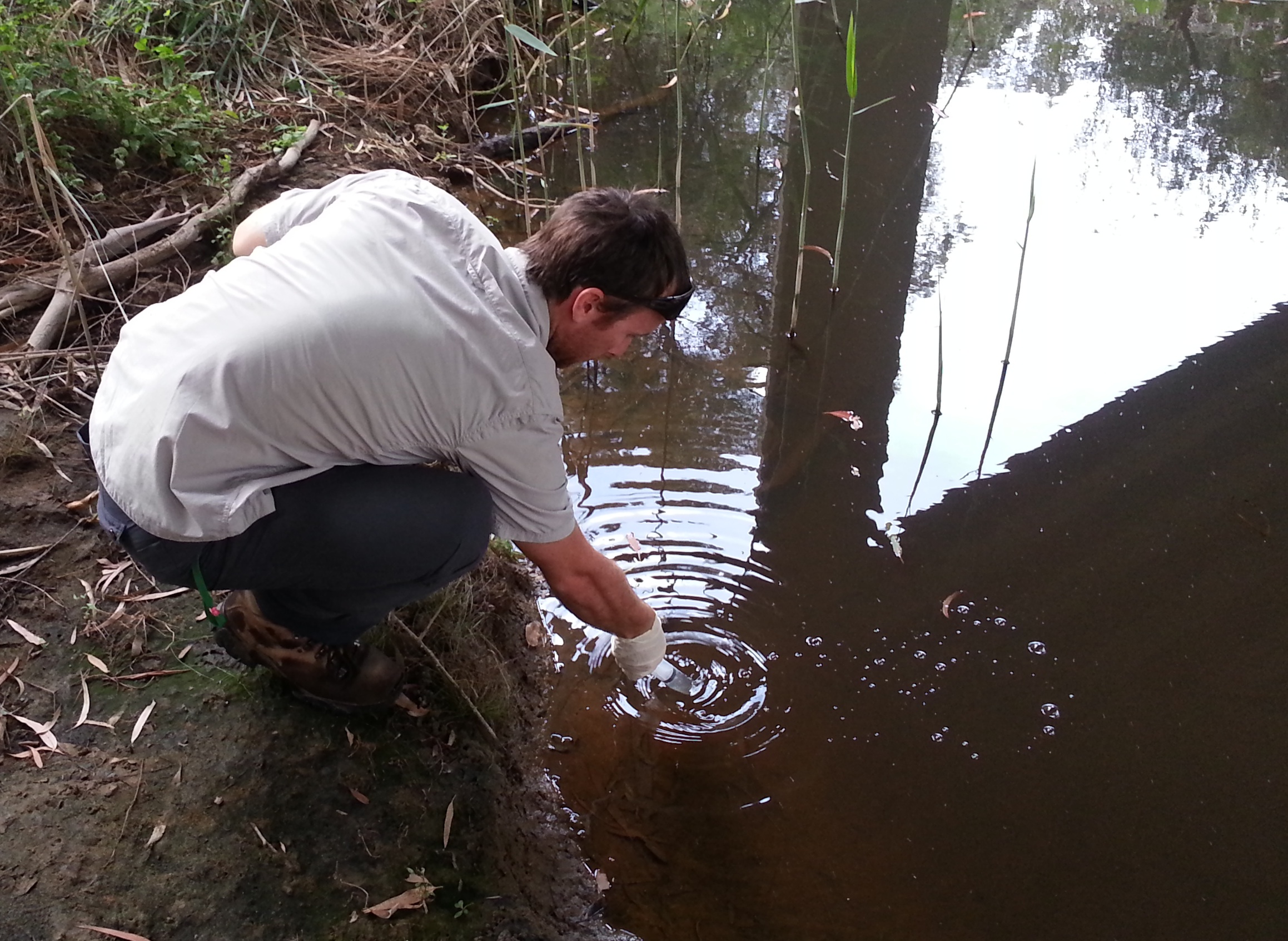
One promising new approach to species monitoring is the collection and processing of environmental DNA (eDNA): the genetic material shed by organisms into their environment. Such surveys are particularly useful in aquatic settings, where eDNA is ubiquitous and relatively easy to collect. Costs of DNA sequencing are dramatically decreasing, making these surveys an efficient monitoring method for many systems.

But as with any method, eDNA surveys are not perfect. Despite DNA extraction and lab protocols being continuously refined, there are still some chances for false negative and false positives. In fact, eDNA surveys present the added challenge that errors can be generated at multiple levels. For instance, a water sample may fail to capture eDNA material from the target species present in the environment. But, even if target eDNA is captured in the sample, it may not be detected during PCR (Polymerase Chain Reaction, the eDNA detection test conducted in the lab). Both of these would give you a false negative.

In contrast, you can get false positives by contamination at the water sample level in the lab or in the field (e.g., DNA of the target species is truly present in the water sample, but it results from contamination by the person undertaking the sampling), or at the PCR level (due to issues when handling samples in the lab). Another feature to consider when analysing or interpreting data is that eDNA surveys often adopt a nested sampling protocol, with several water samples collected, and several PCRs conducted per water sample. PCRs conducted on the same water sample share some dependence, as the chance for false negatives and/or false positives depends on what happened at the water sample level.

In our paper “Dealing with false positive and false negative errors about species occurrence at multiple levels” we present work that dealt with this kind of data. We were interested in analysing records from eDNA surveys for 4 species of frogs conducted in ephemeral roadside drains around Melbourne (Australia). The combination of the nested structure of data collection and the potential for false negative and false positive errors at two different levels meant we could not directly apply existing modelling tools. So, in our paper we present a generalized model for this purpose. But, as above, the eDNA survey data alone were not enough to resolve the ambiguities caused by having false positive and false negative errors. We needed extra information. In our study, we used additional data from an unambiguous detection method (aural surveys), and results from two calibration experiments in which blank water samples were processed (one conducted at the water sample level, the other at the PCR level).

We found that, because we were dealing with errors at two levels, we needed at least two extra sources of information for model parameters to be unambiguously estimated. Not all combinations of data fully resolved the uncertainties. Combining eDNA data with the unambiguous records and the calibration experiment at the PCR level did. And so did combining eDNA data with the two calibration experiments. Of course, having all those data available to us, the best approach was to combine it all… so we ran an integrated analysis of the full lot!

Profile Likelihoods… and a Word of warning about Standard MCMC Methods

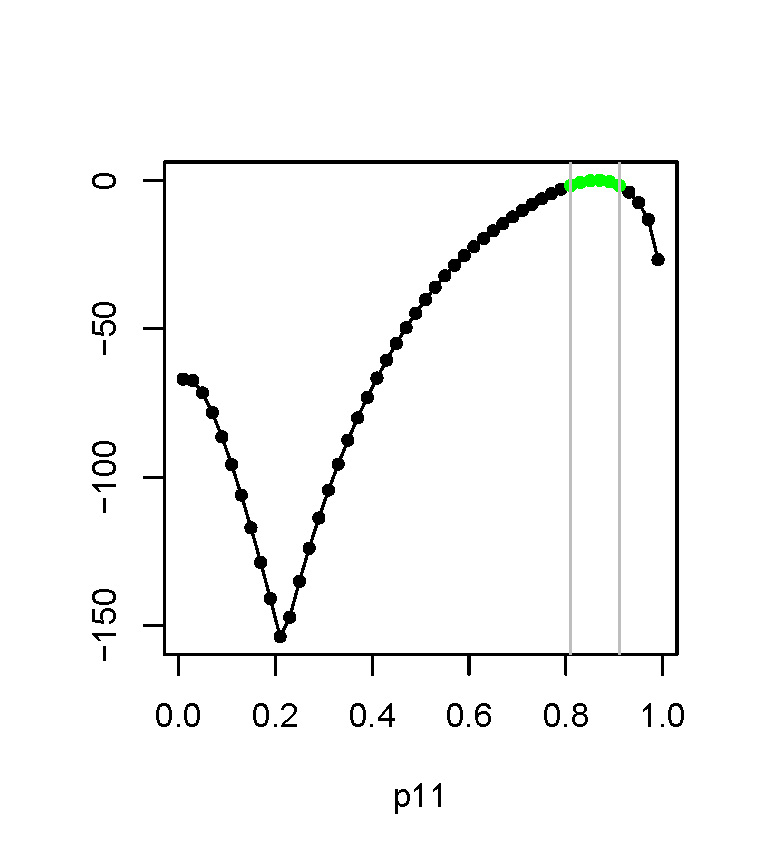
We conducted our model fitting by constructing profile likelihood functions. This is a useful (but underused) technique, and we hope our paper serves as an illustration of its value. So, how does this method work? Say we’re constructing the profile likelihood function for a model parameter theta. What we do is sweep through the potential values of theta and assign to each of them the value of the likelihood function, maximized with respect to all other parameters in the model. From a profile likelihood function, we can compute confidence intervals by slicing the function at a given distance from the maximum. This may sound a bit technical, but it is not hard to apply in practice (we promise!).

We chose this approach for fitting because the likelihood function is bumpy in this model (this is the reflection of the ambiguity in parameter values I mentioned before). Even where additional data are available to resolve parameter uncertainties, there is a risk that standard maximum likelihood optimization methods will get stuck in local maxima, giving wrong parameter estimates; our profile likelihood approach avoids these problems.

And it is worth noting that Bayesian model fitting with standard tools (e.g. BUGS, JAGS, STAN) runs similar risks. We conducted tests (see the appendix of our article) and found that analyses may appear to have converged but MCMC chains can be “stuck” exploring only a fraction of the true posterior distribution (the wrong “bump”). So, I’ll leave it here with a recommendation: run a good number of chains when using MCMC methods, as this can help diagnose identifiability issues (just as it is recommended to rerun analyses with different starting values when applying maximum likelihood estimation via numerical optimization).

To find out more read our Methods in Ecology and Evolution article ‘Dealing with false-positive and false-negative errors about species occurrence at multiple levels’.