I’m Stanislas Mahussi Gandaho, at the Laboratory of Applied Ecology, University of Abomey-Calavi, in Benin. Pablo Palencia from the University of Oviedo and Biodiversity Research Institute in Spain and I wrote ct, an R package for camera trap data, which we describe in our new article.
Why we built ct
Camera traps are cheap to run and they record animals that people rarely see, including those active at night, so many wildlife surveys now rely on them. R already has excellent packages for analysing the results, but each covers one part of the job and expects data in its own format. Moving data between them takes time, and a consistent interface makes the work much easier.
We built ct on tidyverse principles. The package covers routine work, such as reading labels from image files, correcting camera clocks, removing repeat detections, and calculating diversity and activity overlap. The ct package works with data in the Camtrap Data Package (Camtrap DP) format, as well as data in other formats that can be readily adapted to its functions.
Moreover, ct estimates population density and also answers questions that had few tools at all. Does one species react when another passes? Do animals change their active hours between seasons? Where was a species detected? We wanted to answer these from the same data used for everything else, so we added three analyses.
Comparing density estimates
Many species have no markings that let us recognise individuals, and several methods now estimate density without doing so. They rest on different assumptions, so comparisons of these methods suggest applying more than one to the same data.
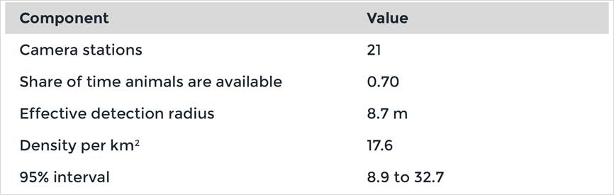
ct brings six density and abundance estimators together: the random encounter model, camera trap distance sampling, three methods based on time, space and instantaneous counts, and the random encounter and staying time model. Each has helpers that prepare its inputs from the same cleaned records. We document what each one builds on and how it calculates uncertainty. We also rewrote the step that calculates uncertainty in distance sampling, which now runs more than 200 times faster in our duiker example.
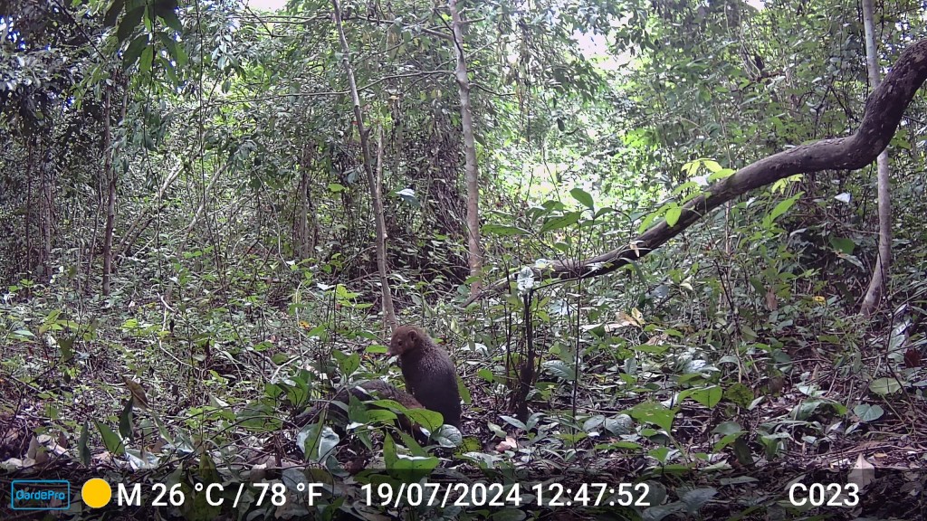
Each method also needs data that only the field can provide, such as animal distances or video with a marked area on the ground. We advise choosing your estimators before the cameras go out, because one design can support several of them. Table 1 shows the distance sampling output for Maxwell’s duikers.
Does one species react to another?
Activity overlap tells you whether two species keep similar hours. It cannot tell you whether one responds to the other at the same place. Models that capture these reactions exist, but they need long surveys and specialist software.
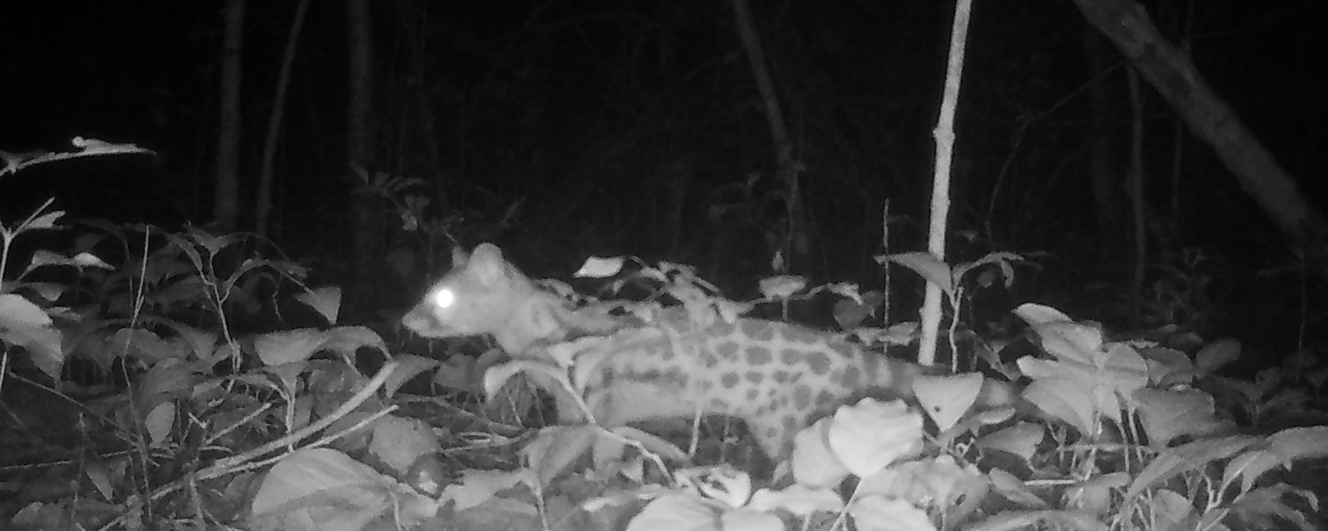
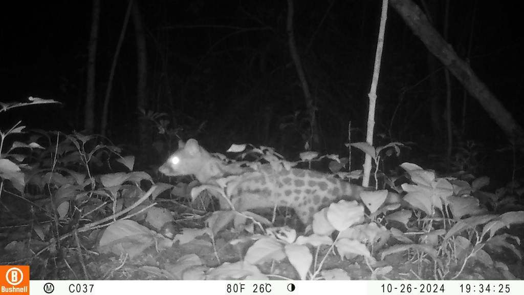
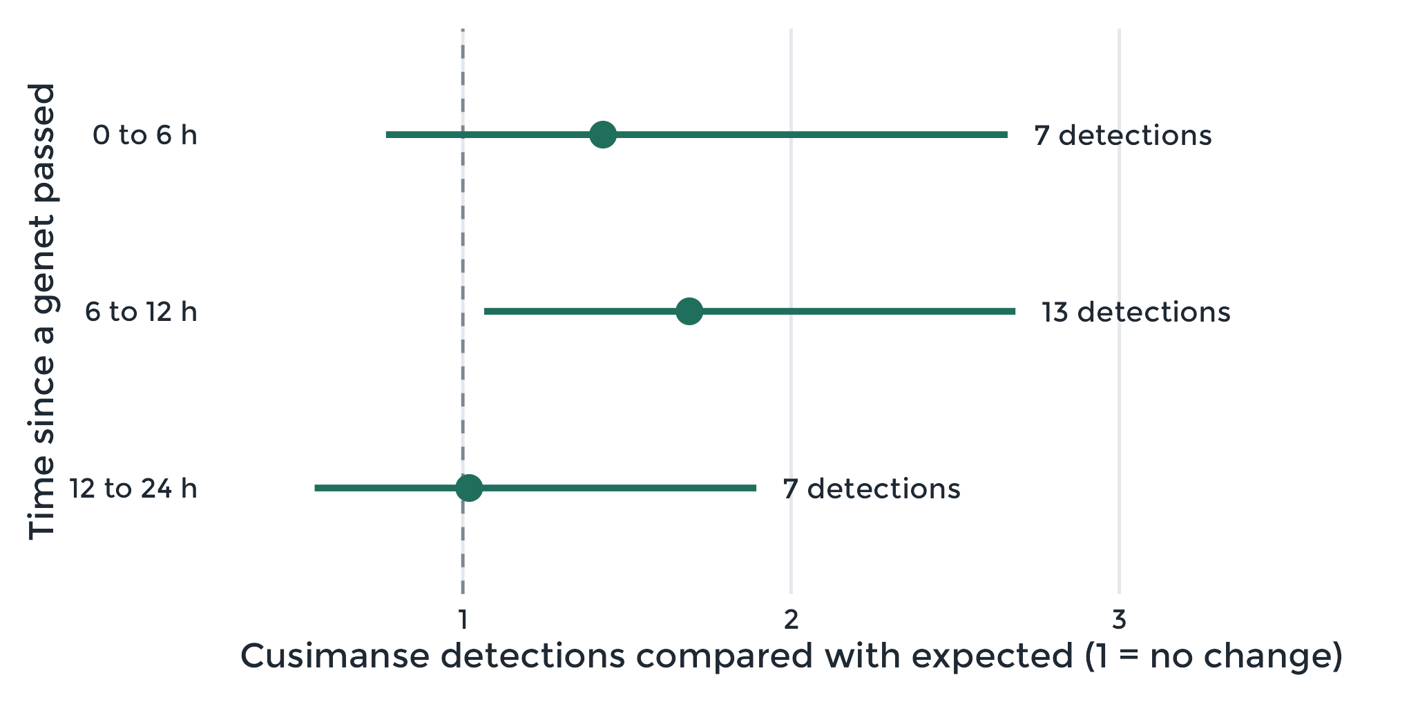
Our encounter response model asks a simpler question. After one species passes a camera, do detections of a second species on that camera rise or fall, compared with what we would expect at that time of day and season? In Lama Classified Forest in Benin, we detected cusimanses about 1.7 times as often as expected in the 6 to 12 hours after a genet passed (Figure 1).
This example rests on few detections, so we treat it as exploratory. It shows an association and does not prove interaction, because a resource that attracts both species could produce the same pattern. In our simulations, with about 200 detections of the second species over 1,200 camera days, the model picked up a doubling of its detection rate in about 9 surveys out of 10.
When animals are active, and where
The temporal shift analysis measures how a species’ active hours change between two periods, such as seasons. In our data from Benin, mona monkeys started and stopped their activity earlier in the rainy season, with the middle of their active period about an hour earlier (Figure 2).
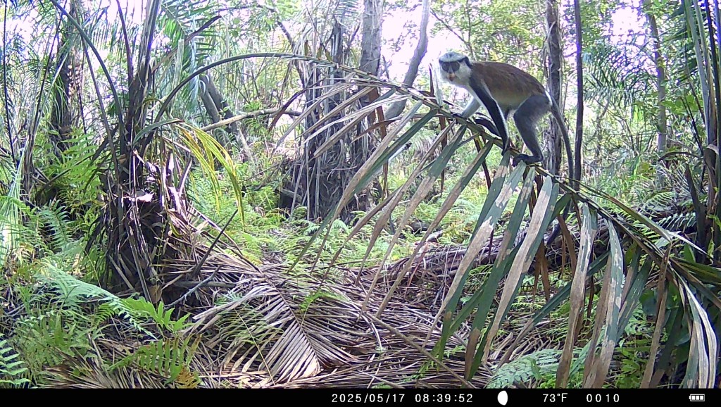
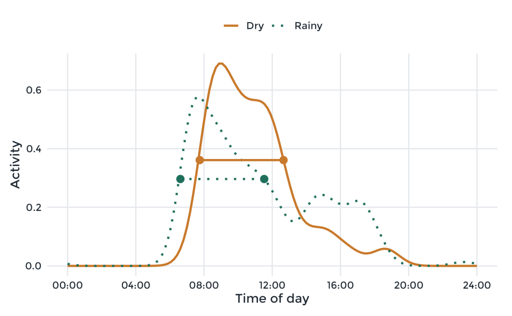
Figure 2: Daily activity of mona monkeys (left) in the dry and rainy seasons (right). The horizontal segments mark the active period in each season, measured at half of the peak. Data and photos from Gandaho et al. (2026).
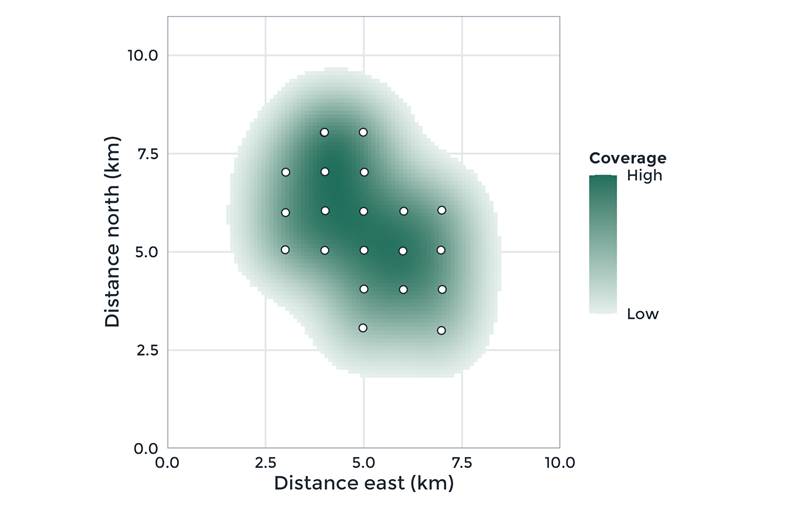
The spatial coverage analysis turns detections into a smoothed map of where a species was recorded. We show it with Maxwell’s duikers in Taï National Park, Côte d’Ivoire (Figure 3). The map describes where cameras detected the species.
Try it, and tell us what breaks
ct is free on CRAN, with documentation and source code online. To install it, run install.packages(“ct”) in R.
Our next studies will test the encounter response model when a shared resource attracts both species and compare the density estimators using one common measure of precision. If ct fails on your data, please open an issue. The work was funded by the R Consortium.
Read the full paper here.

