Post provided by Guillaume Latombe and Melodie A. McGeoch

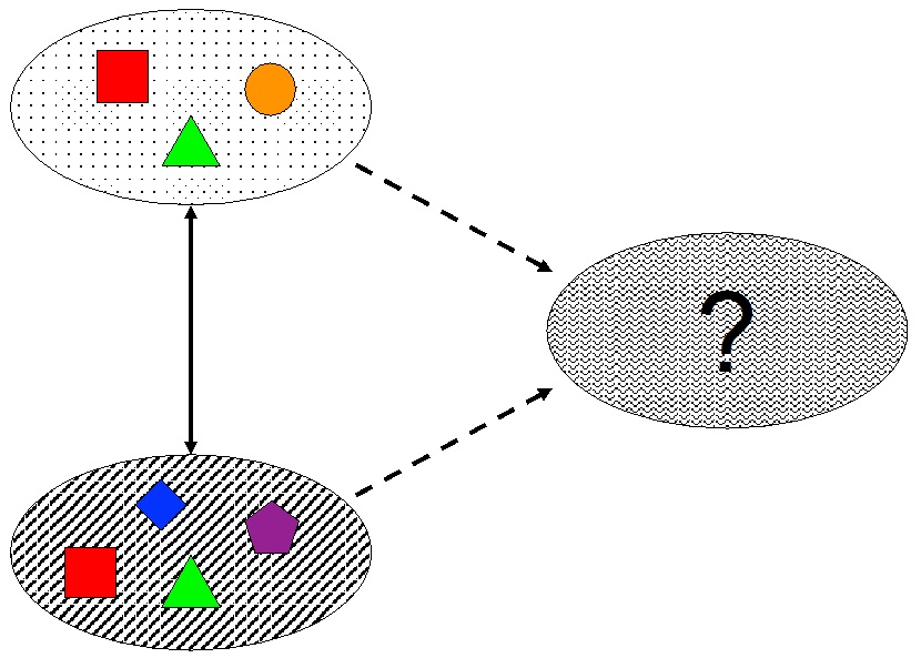
Understanding how biodiversity is distributed and its relationship with the environment is crucial for conservation assessment. It also helps us to predict impacts of environmental changes and design appropriate management plans. Biodiversity across a network of local sites is typically described using three components:

1. alpha (α) diversity, the average number of species in each specific site of the study area
2. beta (β) diversity, the difference in species composition between sites
3. gamma (γ) diversity, the total number of species in the study area.

Despite the many insights provided by the combination of alpha, beta and gamma diversity, the ability to describe species turnover has been limited by the fact that they do not consider more than two sites at a time. For more than two sites, the average beta diversity is typically used (multi-site measures have also been developed, but suffer shortcomings, including difficulties of interpretation). This makes it difficult for researchers to determine the likely environmental drivers of species turnover.

We have developed a new method that combines two pre-existing advances, zeta diversity and generalised dissimilarity modelling (both explained below). Our method allows the differences in the contributions of rare versus common species to be modelled to better understand what drives biodiversity responses to environmental gradients.

Quantifying Species Turnover beyond Pairwise Assemblages – Zeta (ζ) Diversity

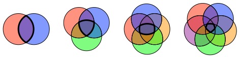
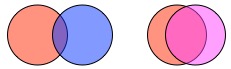
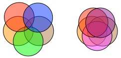
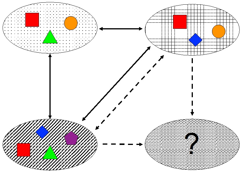
Zeta (ζ) diversity, the number of sites shared by multiple assemblages of species, has recently been proposed as a way to overcome the limitations of traditional biodiversity metrics. Zeta diversity can be divided into ζ₁, the average number of species per site (i.e. alpha diversity), ζ₂, the average number of species shared by any two sites (i.e. beta diversity), ζ₃, the average number of species shared by any three sites, and so on until the maximum number of sites is reached (the number of sites as subscript is referred to as the “order” of zeta). Low orders of zeta capture the contribution of all (well… most) species in the community to turnover. High orders of zeta only capture the more widespread (common) species since, by definition, rare species cannot be shared by many sites. So, zeta diversity necessarily declines as the order of zeta increases.

The rate of decline and form of the decline can vary though, and this provides more information on the processes structuring communities and the distribution of biodiversity than beta diversity alone. In particular, it distinguishes between turnover in rare and common species.

For example, an exponential decline in zeta diversity implies that the ratio ζ_i/ζ_i-1 is constant. From this, we can tell that the chance of finding a common species in a new site is the same as the chance of finding a rare species, meaning that species are randomly distributed amongst sites. By contrast, if the ratio ζ_i/ζ_i-1 increases with the order of zeta, then the chance of finding a common species in a new site is higher than the chance of finding a rare one.

Explaining and Predicting Pairwise Beta (β) Diversity – Generalised Dissimilarity Modelling (GDM)

Generalised Dissimilarity Modelling (GDM) is a regression method to predict beta diversity measures from environmental differences and the distance between sites. Since it is a predictive approach, it assumes that species turnover increases with environmental difference and spatial distance. Also, because it is based on measures bounded between 0 and 1, the relationship between beta diversity and the environmental difference (and distance) must be curvilinear. We accommodate these two constraints by using a generalised linear model (GLM) and forcing the signs of the coefficients to be positive.

In addition to these two constraints on the relationship between beta diversity and environmental difference and spatial distance, GDM takes note of the fact that the environmental difference between sites may have a different impact on species turnover depending on the value of the environmental variable. For example, a small difference in precipitation is likely to have a bigger impact in dry environments than in wet ones. The environmental variables must therefore be non-linearly transformed prior to applying the GLM. To do so, GDM uses I-splines. The non-linearities in the I-splines then inform on where difference in the environment matters. The beauty of GDM is that in practice this transformation does not need to be determined a priori, independently of the GLM. Instead, both the computation of the I-splines and the GLM are determined simultaneously.

GDM has several useful applications, including survey gap analysis, determining where sample activities should be prioritised, and predicting species composition in unsampled sites.

Combining Zeta Diversity and GDM to Produce Multi-Site Generalised Dissimilarity Modelling (MS-GDM)

Given that zeta diversity captures more aspects of turnover than beta diversity, and that it can be used to compute several other common measures of biodiversity, extending GDM to use zeta (i.e. Multi-Site Generalised Dissimilarity Modelling; MS-GDM) is a logical step forward. Since high orders of zeta are determined by more widespread (i.e. common) species and that the distribution of rare and common species can be driven by different environmental variables, we expect different variables to explain different orders of zeta diversity. This sort of information can be invaluable to people making conservation and/or management decisions.

MS-GDM may also improve survey gap analyses by predicting where additional rare or common species should be expected. It can impose more constraints on the algorithms used to predict species composition too, so it could improve the accuracy of these models.

GDM can be adapted for application to multiple sites quite easily. We just need to consider a measure of dispersion for the environmental variables of multiple sites instead of the difference between two sites. For a given number of sites, the most intuitive measures are the mean and the maximum of the pairwise difference between them sites, but other measures of dispersion may also be appropriate (although their effect still has to be assessed).

Multi-Site Generalised Dissimilarity Modelling in Action

We applied MS-GDM to bird assemblages in 25 x 25 km and 100 x 100 km cells over Australia. As well as this, we implemented an alternative to the combination of I-splines and GLM. To do this, we used Shape Constrained Additive Modelling (SCAM), which are similar to the well-known Generalised Additive Modelling (GAM), but can impose monotonic increase or decline to the splines.

SCAM-based MS-GDM does not accommodate the fact that the rate of change in species composition can vary along wide environmental gradients, but SCAM offers more flexibility in the modelling of zeta diversity than GLM. So, SCAM-based MS-GDM should perform better than I-spline-based MS-GDM over small areas with a narrow range of environmental variables, for which the I-splines would be linear. For bird assemblages over the Australian continent, I-spline-based MS-GDM are non-linear and so they outperform SCAM-based MS-GDM.

Our results showed that temperature was the main predictor for high orders of zeta, i.e. widespread species, especially near the extremes of the temperature range. By contrast, precipitation was the main predictor for low orders of zeta, especially in dry areas. Although it would require further ecological analysis, a potential explanation is that changing patterns of precipitation may limit rare species distribution by affecting food resources, whereas common species are more likely to find spatial refugia in wet areas.

Understanding how different environmental variables drive the turnover of common and rare species may have important implications for conservation planning, for predicting the impacts of climate change on biodiversity, and for understanding the consequences of turnover for ecosystem function. MS-GDM may provide more information to help make difficult decisions in these important areas.

To find out more about MS-GDM, read our Methods in Ecology and Evolution article ‘Multi-site generalised dissimilarity modelling: using zeta diversity to differentiate drivers of turnover in rare and widespread species’.

This article is part of the ‘Technological Advances at the Interface between Ecology and Statistics’ Special Feature. All articles in this Special Feature are freely available for a limited time.