Post provided by KATHI IRVINE and TOM RODHOUSE

Or better yet, this post could be named ‘Our Cathartic Journey to Convince Ecologists to STOP Using the Midpoint Values for Analysing Plant Cover Classes’. Our work picks up where another recent Methods.blog post (Stuck between Zero and One) and Methods in Ecology and Evolution article (‘Analysing continuous proportions in ecology and evolution’) by Douma and Weedon left off. They introduced the benefits of using beta and Dirichlet regression. We’re going to tackle the sticky wicket of ordinal data. So, what should you do if you assign a range (like 0.2 to 0.3) instead of record a value (like 0.22) for a continuous proportion?

What is Ordinal Data?

It’s probably a good idea to start by defining the type of data we’re talking about. The best example is from plant surveys. Biologists visually assess the percentage of a pre-defined area covered by a certain plant species. They then record a ‘cover class value’ as an estimate of abundance. Each cover class value corresponds to the percentage of the area that is taken up by the plant in question (e.g., record a 0 for 0%, record a 1 for >0-5%, record a 2 for >5-25%, …, record a 6 for >95%).

In statistical speak, cover class data are an example of ordered categorical or ordinal data. Ordinal data are composed of categories that have an inherent order to them. Back to the plant example, cover class 1 is less than cover class 2 which is less than cover class 3, etc. Back in 2000, Guisan and Harrell suggested that cumulative links models should be used to analyse these data. But biologists continue using the midpoint values as the response variable in a multiple linear regression. For example, if cover class 1 goes from 0 to 5% cover, they would use 2.5 as the response. There are many reasons why we think this is a bad idea (see Sect. 1.3 of ‘Using the beta distribution to analyse plant cover data’).

Why Don’t People Use Ordinal Statistical Models?

I suspect the reluctance to change is because of the strong desire to understand how the environment or management actions are affecting mean percent cover. This is an elusive interpretation when using cumulative link models though.

In a cumulative link model, we should be interpreting things in terms of the odds of moving into a higher cover class category… say what?!? Underlying this interpretation is an assumed logistic or Gaussian distribution that is discretized (or cut-up into categories). So rather than thinking about how the ‘odds’ of invasive weed cover might change after a fire, we can think about a shift in the latent mean of invasive weed cover pre- and post- fire. But this still doesn’t quite cut it because we know that percent cover, even after applying a logit transformation, tends to be skewed (lots of plots in high cover classes and/or low cover classes). But to assume a symmetric distribution like Gausssian for the biological variable of interest – percent cover – seems weird.

A Proposed Solution to Bridge the Gap to Mean Percent Cover

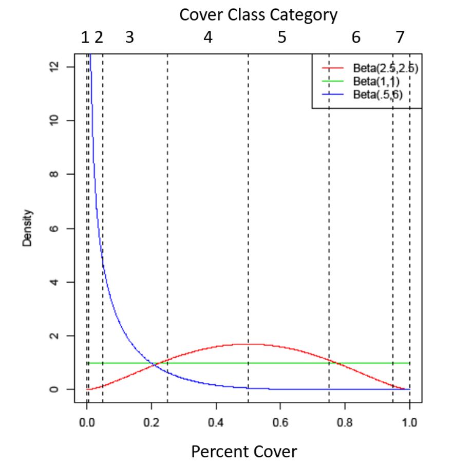
So then, based on our previous dabbling into determining sample sizes for sagebrush steppe monitoring, an interesting twist emerged. What if, instead of using a logistic or Gaussian distribution, we assume a beta distribution? The figure you can see on the left shows some examples of the crazy shapes that the beta distribution can take on within the unit interval. It clearly provides a lot of flexibility. In this figure, the logistic on the percent scale is the same as the uniform distribution (again the assumed latent distribution in a classic ordinal model). This green flat line is definitely not as exciting, in our opinion, as what the beta can handle.

There’s deep historical literature on using the beta distribution to analyse plant cover, but it hasn’t really caught on… yet. It turns out that thresholding the beta distribution with the a priori cover class scheme gives you the interpretation you want and produces less uncertainty. You can do this with our Ordinal Zero Augmented Beta Model (or OZAB for short).

The ‘Z’ part of the OZAB model directly acknowledges that the ‘zero-cover’ class contains information that helps us figure out why a species is absent or why it may occur in certain places (its distribution). This information would be ignored if you were using a cumulative link model. Those models don’t really “care” about the lowest category any more than the middle or highest category. But biologically, it makes sense to consider that the processes determining where a species lives are probably different to those that contribute to its growth. By using the zero-augmented beta distribution we can explore patterns in a plant’s distribution separate from abundance or growth.

Another great thing about making the most of the beta distribution is the connection to a measure of spatial aggregation. This may change over time or be related to measurable environmental factors. In fact, you could extend our model to allow for environmental factors to influence the spatial aggregation and/or precision parameter in the beta distribution. This is an untapped arena for investigation in ordinal ecological datasets.

In ‘A cohesive framework for modeling plant cover class data’, we expand the OZAB in detail. It accounts for true and false zeros, misclassification of cover classes, multiple species and hierarchical sampling designs.

One aspect that is under-appreciated in plant surveys (at least when compared to wildlife surveys) is that a species could be present at trace amounts but be recorded as a 0 – a detection error. Also, observer error could lead to a plant being included in a ‘recorded-cover class’ incorrectly. Our Ordinal Zero Augmented Beta with Errors Model (OZABE) handles this issue. If observation errors are a concern, multiple independent observations for each plot are required. Not necessarily for all plots though – as we found in the case of beta regression with observation errors. Check out our paper supplements and give the models a try!

To find out more about OZAB and OZABE, read our Methods in Ecology and Evolution article ‘A cohesive framework for modeling plant cover class data’