Post provided by JAMES WEEDON & BOB DOUMA

Chinese translation provided by Zishen Wang

這篇博客文章也有中文版

Imagine the scene: you’re presenting your exciting research results at an important international conference. Being conscientious and aware of statistical best-practice and so you’ve included test statistics and confidence intervals on all your result figures. Not just P values! Some of the data you are presenting involves the proportion of leaf surface damaged by an insect herbivore under different treatments. You finish your presentation (on time!) and there’s time for questions. From the audience a polite but insistent colleague asks: “Your confidence interval for that estimate goes from -0.3 to 0.5… how should we interpret a negative proportion of a leaf?”.

Someone chuckles. As you nervously flick back to the slide in question, you mutter something about the difference between confidence intervals and point estimates. You start to feel dizzy. A murmur of confused voices slowly builds amongst the audience members. In the distance, a dog barks.

How can you avoid this?

Proportional Data in Ecology and Evolution

Many kinds of quantities that ecologists and evolutionary biologists routinely measure are most conveniently expressed as proportions. In many cases these proportions are derived from counts. The data are based on discrete entities that can be assigned to two or more classes: success or failure, male or female, invasive or non-invasive. In other cases the proportions are derived from continuous measurements: the proportion of time an animal spends on different activities;  percent cover of a plant functional type in a vegetation survey quadrat; allocation of total plant biomass to different organs and tissues. What these data types have in common is that they can only take values between zero and one. Negative values, or values greater than one, don’t make any sense.

This can cause problems if you use regular statistical tools to analyse this kind of data. Linear regression, ANOVA and other methods which are the typical elements of biologists’ statistical training, assume that the response variable can be modelled with a Normal distribution. Normal distribution is defined for values ranging from negative to positive infinity. So it’s not really an appropriate choice for modelling quantities, such as proportions, that are constrained to an interval. Predicted values and confidence intervals from your model are very likely to include values outside the interval. Residuals will be strongly related to predicted values. These are all signs of a mis-specified model that can lead to suspect inferences.

Models for Proportional Data

When proportions are derived from counts, logistic regression and its extensions are appropriate models. These techniques are well established and they’re covered in most introductory textbooks.

When proportions come from continuous measurements (e.g. percent cover, fraction time spent, biomass fraction) there’s less consensus on best practice. A commonly used solution is to apply a transformation to the data which maps values from the zero to one interval to the entire real number line. After transformation the usual suite of statistical models, assuming a Normally distributed response, can be applied. For many years the arcsine transformation was advised, but analyses by David Warton and Francis Hui have demonstrated that the logit transformation is a better option.

In recent years, techniques have been developed that avoid this transformation step.  These methods replace the Normal distribution with a probability distribution that’s explicitly constrained to the zero to one interval. In cases where proportional data are derived from continuous (non-count) measurements the beta and Dirichlet distributions are the ideal candidates.

Despite being first introduced more than a decade ago, beta and Dirichlet regression are rarely used by ecologists and evolutionary biologists. This is surprising, since up to 15% of papers in ecology deal with some kind of proportional data. In ‘Analysing continuous proportions in ecology and evolution: A practical introduction to beta and Dirichlet regression’ we provide a resource for ecologists and evolutionary biologists who are interested in applying these techniques to their data analysis problems. It’s specifically aimed at people who don’t feel comfortable delving into the disparate, and quite technical, literature around these topics.

Beta and Dirichlet regression let you model proportional data on their original scale, using continuous or categorial predictors. Beta regression is used for simple proportions, and Dirichlet when there are more than two possible components. For example, when modelling plant biomass allocation to different organs you’d use Dirichlet. If you were to analyse leaf damage data, you’d use beta regression.

There are extensions available for hierarchical data structures and variable dispersion. With these, it’s possible to perform analyses just like the familiar techniques of (multiple) linear regression, ANOVA, ANCOVA, mixed-effects. But, they also allow for the special properties of proportional data.

If you’re familiar with Generalized Linear Models (GLMs) then the fitting and interpretation of beta and Dirichlet regression models will be easy to understand. A model for the relationship between predictor variables and parameters of the response distribution is specified via a link function. This ensures that all predictions are constrained to values that are meaningful.

Below, you can see the main differences between normal linear regression (left) and beta regression (right) for a simple case of analysing a proportional response (constrained between 0 and 1) and a predictor variable. The data are shown as blue points. The best fit line for each case is the dashed red. The predictive distribution at a range of values for the predictor variable are plotted as grey density distribution.

It’s clear that the beta regression provides a more appropriate model for this data. Both the predicted values and the associated distribution are constrained between 0 and 1. The normal linear regression predicts values greater than 1 or less than zero. This is nonsensical when dealing with proportional data.

A more complex example using Dirichlet regression is shown below. The data come from a real study that analysed the allocation of biomass to different plant tissues through time for two species under different nutrient regimes (see here for a subsequent reanalysis). Given the wide range in possible plant sizes, it made sense to standardize biomass measurements as proportions of total biomass per individual plant. Since the proportions of the total have to add up to one, the different components have a complex interdependence that needs to be accounted for in the analysis. Dirichlet regression accounts for this interdependency between responses.

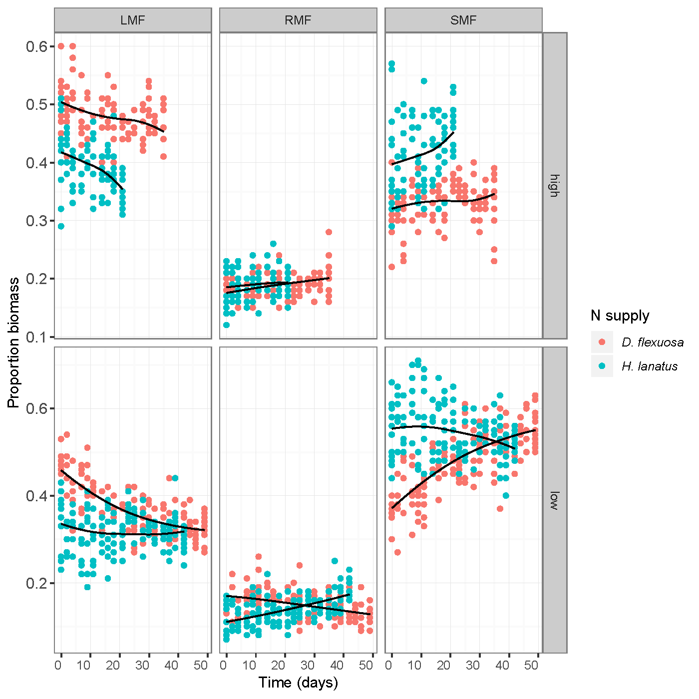
This example shows biomass partitioning over time to leaves (LMF), roots (RMF) and stems (SMF) for two plant species (Holcus lanatus and Deschampsia flexuosa). They were grown in two contrasting nutrient regimes (rows, low vs high). Black lines indicate model predictions. For each species x nutrient combination these sum to one across the columns. Dirichlet regression makes this possible. With other methods, we could end up with models showing over 100% of the plant’s biomass going to the leaves.

A User’s Guide to Analysing Proportions in Ecology and Evolutionary Biology

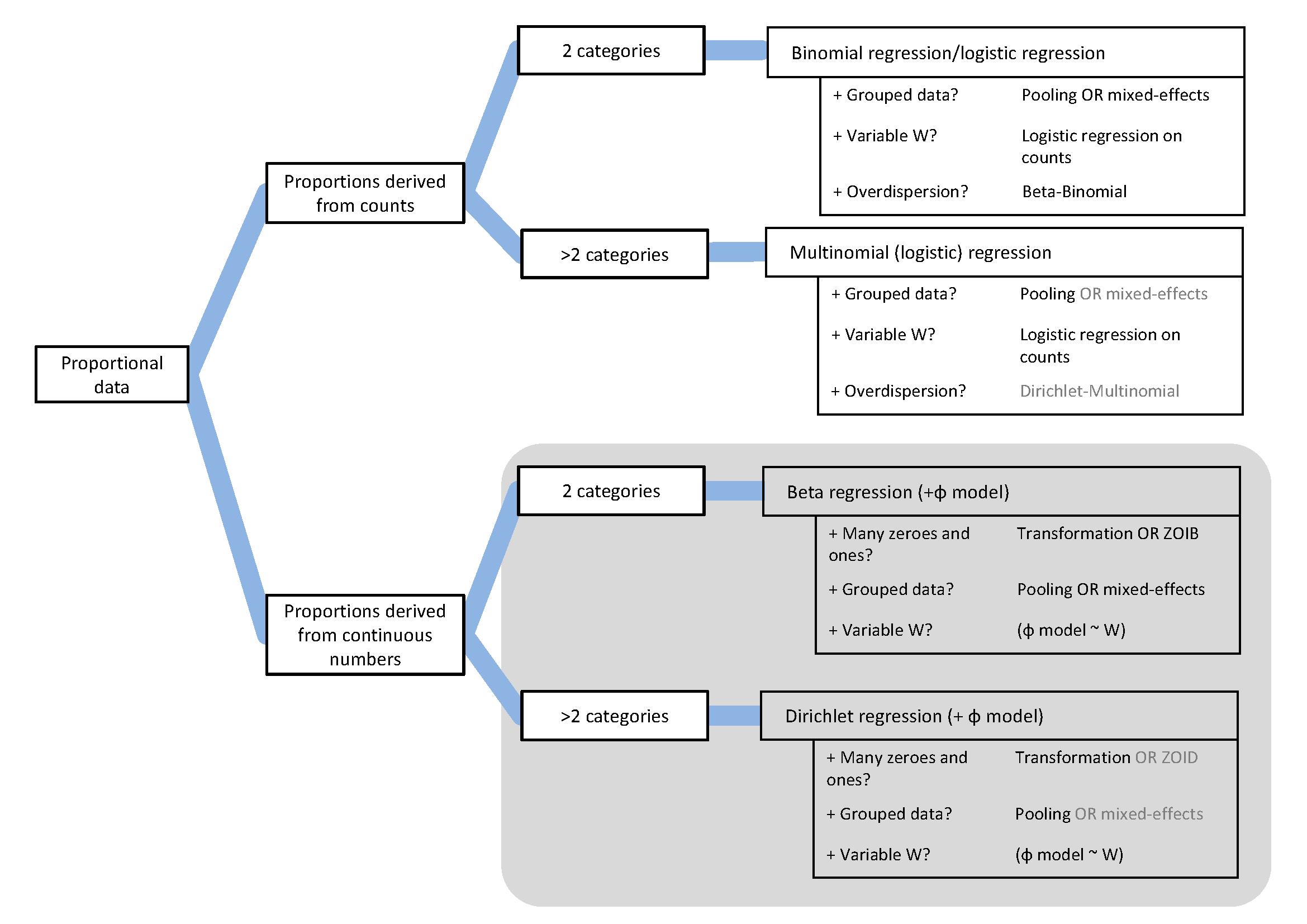
‘Analysing continuous proportions in ecology and evolution: A practical introduction to beta and Dirichlet regression’ aims to provide a non-technical introduction to these techniques for practitioners in ecology and evolutionary biology. We keep the technical details to a minimum and focus on practical advice. We start describing different kinds of proportional data and present a decision tree to help practitioners match properties of their data and experimental design to the right analysis.

We give non-technical descriptions of beta and Dirichlet regression and cite examples of their use in ecology and evolution research. We also describe the most important extensions for the types of data that are used in ecology and evolutionary biology (including hierarchical (nested) data, and zero inflation).

To make the article as helpful as possible, and to bridge the gap between reading about analyses and applying them to real problems, we provide three detailed case studies. For all three we provide data and annotated R code for full reproducibility; and to provide readers with example code to be adapted to their own analysis problems. Examples include the use of the R packages betareg, DirichletReg, brms and zoib.

Proportional data are common in ecology and evolution. They require specific techniques for their reliable analysis. We hope that our article provides readers with the information and inspiration to start confidently using beta and Dirichlet regression in their analyses.

To find out more about beta and Dirichlet regression, read our Methods in Ecology and Evolution article ‘Analysing continuous proportions in ecology and evolution: A practical introduction to beta and Dirichlet regression’