Post provided by Ané Cloete

What is acoustic spatial capture-recapture (aSCR)?

Estimating how many animals live in a given area is one of the most fundamental challenges in conservation. For species that are easy to see such as large mammals on open plains, for example, this is manageable. But for cryptic species that hide from view, counting them directly is often impossible. This is where sound becomes a surprisingly powerful tool.

Acoustic Spatial Capture-Recapture (aSCR) is a method that allows researchers, wildlife managers, and conservation practitioners to estimate the density and abundance of wildlife populations using sound recordings alone. It is particularly well-suited to species that are hard to see but vocally active — think gibbons calling through thick forest, or tiny frogs with surprisingly loud voices on a mountain slope.

aSCR is an extension of Spatial Capture-Recapture (SCR), a widely used statistical framework commonly deployed with survey technologies like camera traps or DNA sampling. What makes aSCR distinctive is that it swaps physical detections of individuals for detections of their calls. The animal itself never needs to be seen, only heard.

There are two main flavours of aSCR. The first (sometimes called the call-density model) estimates how many calls are being produced per unit area, then converts this to animal density using a separate estimate of how often individuals call. The second (the animal-density model) estimates animal density more directly, but requires that the calls recorded can be matched back to specific individuals, a harder task, as we will see.

What does aSCR need to work?

At heart, aSCR needs two things: an array of microphones spread across the landscape, and a way to know which microphones detected the same call. This spatial pattern of detection, one call heard by multiple devices, is the engine that drives the whole method.

Consider surveying the Cape Moss Frog, a tiny frog that lives on the slopes of Table Mountain. You place a grid of microphones across its habitat, spaced so that a call from any given frog is likely to be picked up by more than one microphone, but not by every microphone in the array. When a frog calls, the pattern of which microphones detected it (and which did not) tells you roughly where that call originated. The more microphones detect it, the closer the frog was to the centre of those detectors. This spatial re-detection of calls is what gives the method its name and its power.

The survey period needs to be short enough that the population can be assumed to be closed, meaning no animals are born, die, or move into or out of the area during the recording. For many species, a single recording session of a fixed duration (for example, a 10-minute window extracted from a longer recording) is enough to meet this requirement. The appropriate length depends on the behaviour of your study species and should be informed by pilot studies beforehand.

Practical considerations matter too. You need to account for the time it takes to set up the microphones and leave the area before analysis begins. Survey design is a discipline in its own right, and getting it right for your species and site requires careful thought, consultation with experts, and ideally, some simulation work in advance.

What data does an aSCR model use?

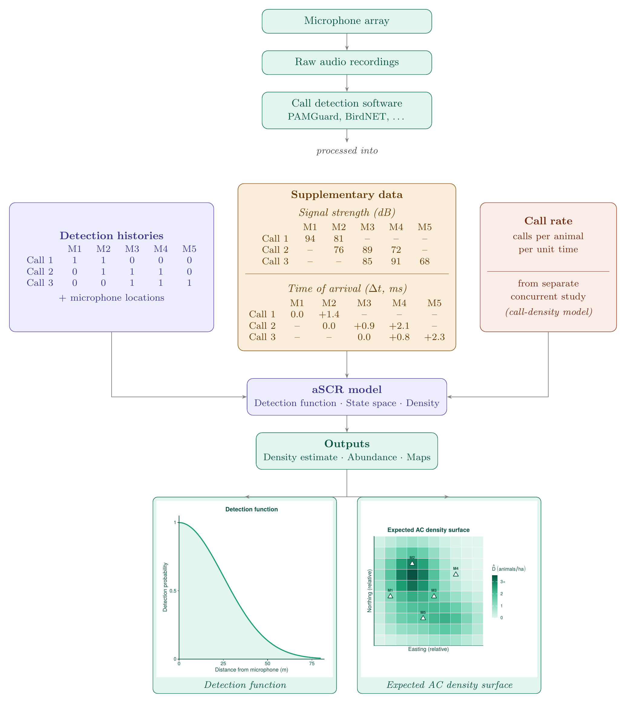
Once recordings are collected, they need to be processed before the model can use them. Raw audio is typically run through specialised passive acoustic monitoring software (tools like PAMGuard or BirdNET) to detect and classify calls, either automatically or with manual checking. From this, a simple record is built: for each detected call, which microphones heard it (a 1) and which did not (a 0). This is called a detection history, and it is the basic input every SCR model needs.

In addition to the detection histories, the model also needs to know where each microphone was located. The combination of detection patterns and microphone positions is what allows the model to reason about where calls came from.

Supplementary acoustic data

Microphones can collect more than just a presence-or-absence signal. Two additional types of data are especially useful and can substantially improve the precision of density estimates.

The first is signal strength, the loudness at which a call was received. Sound fades with distance, so a call received at high volume was likely produced close to that microphone. By comparing the loudness recorded at different microphones, the model can triangulate the likely origin of a call.

The second is the precise time the call arrived at each microphone. Sound travels at roughly 343 metres per second in air, which means a call reaches the nearest microphone a fraction of a millisecond before it reaches the others. These tiny time differences carry a surprising amount of location information. Collecting time-of-arrival data requires that all microphones in the array are precisely synchronised with each other, an important practical consideration when planning a survey.

Call rate and individual identity

The call-density model additionally needs an estimate of how often individual animals call. In other words, their call rate. This is typically measured from a separate study conducted at the same time as the main survey, to ensure conditions are comparable. Without this, the model can estimate the density of calls but cannot convert that into a density of animals.

The animal-density model sidesteps this requirement, but only if calls can be matched back to individual animals. For some species, individual calls have distinctive enough features that identity can be inferred from the recording alone or using a mathematical rule, calls can be assigned to individuals. For many species, this is not possible or cannot be done with sufficient certainty, which is why the call-density model is more commonly used at the moment.

Spatial variation in density

The basic aSCR model assumes that animal density is uniform across the survey area. The same number of animals per hectare everywhere. This is often unrealistic. Where the terrain, vegetation, or microhabitat varies, so will the animals. More advanced versions of the model allow density to vary across space, but this requires collecting environmental data at representative locations across the survey region to help explain that variation.

Core components of an aSCR model

Under the hood, an aSCR model has three working parts that together allow it to estimate density from acoustic data.

How detection probability changes with distance

Not every call that is produced will be detected by a given microphone. A call produced right next to a microphone is almost certain to be picked up; a call produced far away might not be. The relationship between distance and the chance of detection is captured by what is called a detection function, essentially a curve that starts high (near certainty of detection when close) and drops towards zero as distance increases.

The model estimates the shape of this curve from the data itself. This is one of SCR’s key advantages: rather than assuming a fixed detection range, it learns from the pattern of detections and non-detections what range is actually operating in the field. This matters because detection range varies with wind, vegetation density, and ambient noise, conditions that can change between surveys and sites.

Defining the survey area

The model needs to know the region over which animals could plausibly have been detected. This is called the state space or mask and is a defined area that is large enough to include any animal that had a realistic chance of being heard by at least one microphone. Setting this boundary requires some thought: too small, and you exclude animals that genuinely contributed to your detections; too large, and you waste computational effort on areas that could not have contributed any calls.

Estimating density

With a detection function and a defined survey area in hand, the model can estimate how many animals are present per unit area. In the basic model, this is a single number. One density estimate for the whole region. In more complex versions, density can be allowed to vary spatially, producing a map of where animals are more or less concentrated. This is particularly useful for understanding habitat use or identifying conservation priority areas.

What assumptions does aSCR rely on?

Like all models, aSCR works best when its assumptions are met. The main ones to be aware of are:

Animals are not moving much during the survey. The model treats each animal as calling from a fixed location, its activity centre. If animals are moving around significantly, the pattern of detections becomes harder to interpret, and density estimates can be biased.

Calling behaviour is consistent and representative. The model assumes that all individuals have a similar probability of calling during the survey period, and that their calls are detectable. In practice, this is not always the case, some animals call more loudly or more often than others, and for species like gibbons, not all groups call on any given day. This kind of individual variation in calling probability is a known challenge, and accounting for it properly requires more advanced modelling approaches.

Microphones are performing reliably. If some microphones are malfunctioning, waterlogged, or picking up excessive background noise, the pattern of detections will be distorted. Regular equipment checks before and after surveys are important.

The population is closed during the survey. No animals should be entering or leaving the area, or being born or dying, during the recording period. For most short survey sessions, this is a safe assumption.

What kinds of ecological questions can aSCR answer?

aSCR is particularly valuable for monitoring cryptic species. Frogs, nocturnal birds, gibbons, cetaceans, and bats are all good candidates. In each case, passive acoustic monitoring can cover large areas at relatively low cost, and aSCR turns those recordings into rigorous density estimates with quantified uncertainty.

Beyond simple counts, aSCR can reveal where animals are concentrated within a landscape, which habitat patches are used most intensively, and which are avoided. This spatial information can directly inform conservation planning, from reserve design to habitat management.

aSCR is also well-suited to population monitoring over time. Because the method accounts for variation in detection conditions (rather than assuming a fixed detection range), it produces estimates that are genuinely comparable across surveys conducted in different seasons or years. This makes it a powerful tool for tracking population trends.

Where is aSCR heading?

aSCR is a relatively young method and continues to develop quickly. Current research is pushing in a few exciting directions: better ways to handle species where individual identity cannot be determined from calls alone; methods that do not require call rate estimates from separate studies; and tools that make the approach more accessible to practitioners without a statistical background. As passive acoustic monitoring hardware becomes cheaper and more widespread, and as machine learning improves the speed and accuracy of automated call detection, aSCR is likely to become one of the go-to approaches for monitoring elusive wildlife at scale.

If you’d like to know more, here are some useful resources:

• https://bcstevenson.nfshost.com/acre-worksheet.html
• https://anecloete.shinyapps.io/aSCRTut/
• Stevenson, B.C., Borchers, D.L., Altwegg, R., Swift, R.J., Gillespie, D.M. and Measey, G.J., 2015. A general framework for animal density estimation from acoustic detections across a fixed microphone array. Methods in Ecology and Evolution, 6(1), pp.38-48.
• Stevenson, B.C., van Dam‐Bates, P., Young, C.K. and Measey, J., 2021. A spatial capture–recapture model to estimate call rate and population density from passive acoustic surveys. Methods in Ecology and Evolution, 12(3), pp.432-442.