McGill et al. (2006) argued that community ecology had lost its way. Shipley (2010) accused community ecologists of acting like a bunch of demented accountants. Strong words – so what’s the issue exactly?  And what can we do about it?

Their beef was that when studying groups of species and their environmental association, ecologists often were not thinking enough about the reasons for variation across species. (In this post we’ll focus on variation in abundance or in environmental response of abundance across species. We’re interpreting “abundance” loosely – counts, biomass, 1-0, whatever.)  While alternative methods are more readily available nowadays, “accountancy” is still common.

For example, consider a study of the effect of pollution on an assemblage of marine invertebrates (classified to species), and the sorts of multivariate analysis methods currently used to address this type of problem. Current go-to methods are things like PERMANOVA, RDA, manyglm and adonis. Each of these can look collectively at how the assemblage responds to pollution, with some allowance for the possibility of different responses in different species, but none of them looks at why responses differ across species. The analyst might be left sifting through reams of results indicating different responses for different species with little sense for (or means of understanding) why species differ in response.

As scientists we usually want to understand why things happen rather than just documenting them. In the quest to understand why there is variation in a response variable (conveniently, usually written as Y), a common starting point is to look for predictors (X) that might explain the pattern. When studying variation across multiple species, the relevant predictors are commonly referred to as species traits or functional traits. So studying the problem of why different species have different abundance patterns can be as simple as including functional traits as predictors – seems obvious enough. But this is not really a feature of the multivariate analysis literature in ecology, perhaps because the distance-based methods so widely used are not amenable to including predictors on species as well as on sites. It’s not much of a feature of the species distribution modelling literature either, perhaps because of the tendency to do things one species at a time.

Shipley’s CATS model (Shipley et al. 2006, published in Science no less) is one approach to the problem of explaining why some species at a site are more abundant than others. This is not really a multivariate approach; it’s a maximum entropy method intended for observations of abundance of species at a single site, together with functional trait measurements. A paper in the Special Feature for the April issue of Methods (New Opportunities at the Interface Between Ecology and Statistics) shows that CATS is equivalent to fitting a Poisson regression for abundance against functional traits (“CATS regression”, Warton et al. 2015), in a result closely analogous to recent equivalences in presence-only analysis.  Using a regression framework is helpful because it can be used to extend CATS to new problems, for example, a multivariate analysis of data from multiple sites to understand why environmental response differs across species.

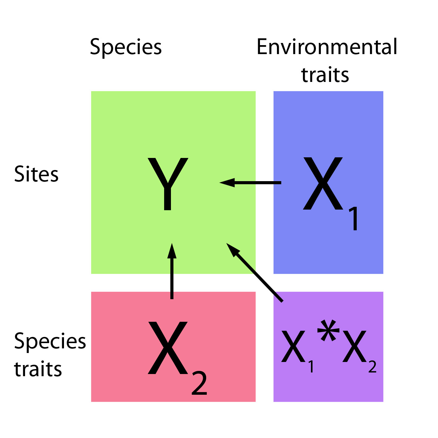
In the multiple site setting the abundance response (Y) is now a matrix and there are two sets of predictors – traits operating on species (X₂) and environmental variables operating on sites (X₁).  We want a model for Y as a function of X₁, X₂, and their interaction. The X₁*X₂ interaction is the important bit, as it shows how interspecific variation in environmental response can be explained by functional traits. This idea has been incorporated into the mvabund package (from version 3.10) – it now has a traitglm function for fitting such models using GLMs, and an anova function for testing for an environment-trait interaction. A brief tutorial is available on the Eco-Stats blog. The main difference from a regular GLM is the use of resampling to account for correlation in abundance between species when making inferences across species.

If this idea sounds familiar and you think you have seen it before, maybe you have.

Some earlier work on studying environment-trait interactions by Legendre et al. (1997) described the “fourth corner problem” as being how to combine the three data matrices (Y, X₁, X₂) to construct a matrix in the “fourth corner” which quantifies the strength of environment-by-trait associations. In a regression framework though, the matrix of environment-by-trait interaction coefficients (X₁*X₂) can be understood as being exactly this fourth corner and, in some situations, the method of Legendre et al. (1997) gives the same results as Poisson regression (Brown et al. 2014, Appendix). So the ideas are closely connected, but there are advantages to approaching the problem using regression (Brown et al. 2014).  One such advantage is the potential to incorporate intra-specific variation into models, hence addressing another criticism levelled at community ecologists (Violle et al. 2012), who by now might be feeling a little defensive…

Or you might have previously seen this idea in a study that used traits to explain differences in species distribution models (Pollock et al. 2012), applied in a generalised linear mixed model (GLMM) to find connections between Eucalyptus species distributions and the extent to which these might be attributable to plant height, specific leaf area, and seed mass (the “LHS scheme”). Or in Jamil et al. (2013), who also used a GLMM and compared their results to a conventional fourth corner analysis. It is worth noting however that the central idea is not wedded to GLMMs or any other type of model – it is simply to use functional traits as predictors in your model as well as environmental variables, and environment-trait interactions as a way to explain interspecific differences in environmental response.  You could probably even apply this idea using a fancy new model like mistnet (Harris 2015), also in the April MEE issue.

Is this all overly complicated? Instead of this weird three matrix stuff, can’t you just measure some aggregate trait quantity at each site (eg. an abundance-weighted trait mean) and regress that against environment across sites? Yes, and in some cases that has connections to Poisson regression too – abundance-weighted trait means can be understood as the sufficient statistics in a CATS regression (Warton et al. 2015), i.e. they are the statistics that are needed to fit a CATS model (as in Shipley 2010). The most important thing to recognise with the trait-mean approach is that changing the response being predicted changes the question being answered. Instead of using traits to explain differences in environmental response across species, you would be using environmental variables to explain differences in trait means across sites. There could also be a statistical cost to this change in strategy – if your data were overdispersed compared to a Poisson, abundance-weighted trait means could be expected to be overly sensitive to the trait values of abundant species, so one could expect some loss of efficiency (eg. bigger se’s).

So will we see a little less “demented accountancy” and a little more trait modelling?  Not everyone needs to know why, so clearly we don’t all need to go there. But enough of us would like to know why that I am hoping we are entering a new phase in multivariate analysis (/SDM)…

References
Austin, M., Nicholls, A. & Margules, C. R. (1990) Measurement of the realized qualitative niche: environmental niches of native Eucalyptus species. Ecological Monographs, 60, 161-177.
Brown, A.M., Warton, D.I., Andrew, N.R., Binns, M., Cassis, G. & Gibb, H. (2014) The fourth-corner solution – using predictive models to understand how species traits interact with the environment. Methods in Ecology and Evolution, 5, 344–352.
Harris, D.J. (2015) Generating realistic assemblages with a Joint Species Distribution Model. Methods in Ecology and Evolution, 6, 465-473.
Jamil, T., Ozinga, W.A., Kleyer, M. & ter Braak, C.J. (2013) Selecting traits that explain species–environment relationships: a generalized linear mixed model approach. Journal of Vegetation Science, 24, 988–1000.
Legendre, P., Galzin, R. & Harmelin-Vivien, M.L. (1997) Relating behavior to habitat: solutions to the fourth-corner problem. Ecology, 78, 547–562.
McGill, B.J., Enquist, B.J.,Weiher, E.& Westoby, M. (2006) Rebuilding community ecology from functional traits. Trends in Ecology and Evolution, 20, 178–185.
Pollock, L.J., Morris, W.K. & Vesk, P.A. (2012) The role of functional traits in species distributions revealed through a hierarchical model. Ecography, 35, 716–725
Shipley, B., Vile, D. & Garnier, E. (2006) From plant traits to plant communities: a statistical mechanistic approach to biodiversity. Science, 314, 812–814.
Shipley, B. (2010) From Plant Traits to Vegetation Structure: Chance and Selection in the Assembly of Ecological Communities. Cambridge University Press, Cambridge.
Violle, C., Enquist, B. J., McGill, B. J., Jiang, L., Albert, C. H., Hulshof, C., Jung, V. & Messier, J. (2012). The return of the variance: intraspecific variability in community ecology. Trends in Ecology and Evolution, 27, 244-252.
Wang, Y., Naumann, U., Wright, S. T. & Warton, D. I. (2012). mvabund – an R package for model-based analysis of multivariate abundance data. Methods in Ecology and Evolution, 3, 471-474.
Warton, D.I., Shipley, B., & Hastie, T. (2015) CATS regression – a model-based approach to studying trait-based community assembly. Methods in Ecology and Evolution, 6, 389-398.