Post provided by Jeff W. Atkins (he/him)

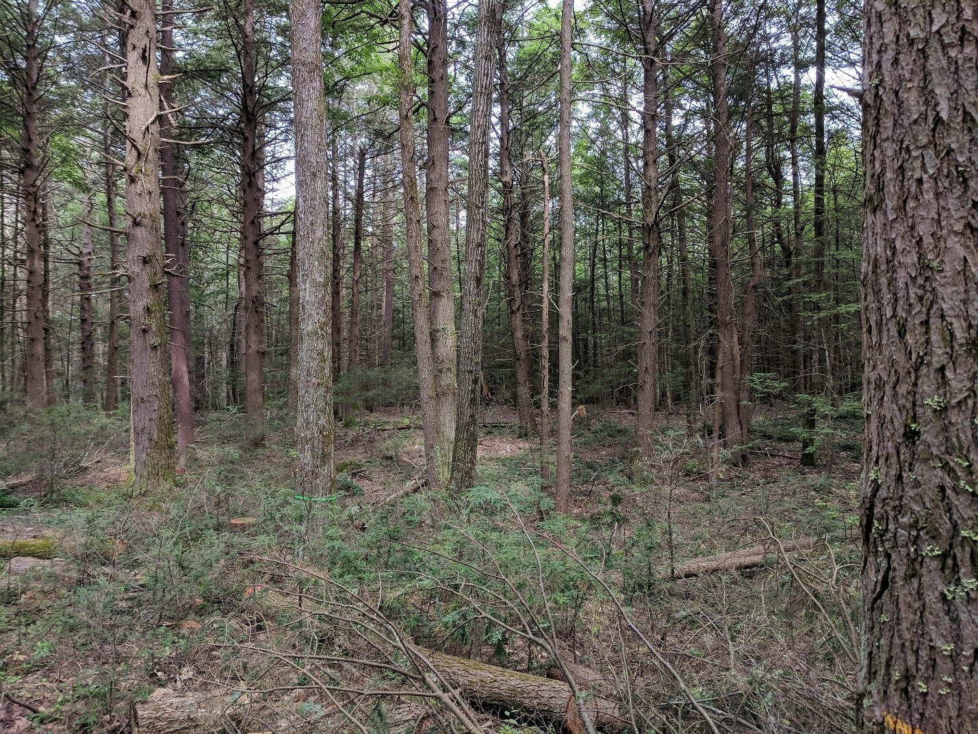
Ecological researchers have adopted light detection and ranging (LiDAR) as a means of quantifying ecosystem structure over the past 25+ years. This is especially true in forest-related research, as LiDAR provides the ability to estimate ecosystem structure with incredibly fine detail, over broad areas. LiDAR can work at the scale of individual trees—for example crown delineation algorithms that identify singular tree canopies—or the stand-level with aggregate structural metrics. In this blog post, Jeff shares insight from he and his co-author’s recent publication “Scale dependency of LiDAR-derived forest structural diversity,” which proposes that using LiDAR requires statistical reassessment to ensure we are measuring what we think we are.

What is LiDAR?

LiDAR is a form of active remote sensing based on the idea that because the speed of light is constant, we can measure distances by bouncing light off objects and measuring the time taken for the signal to return.

LiDAR provides precise and accurate estimates of forest height as well as the ability to create derived, aggregate metrics that describe additional dimensions of forest structure—such as canopy complexity, arrangement, openness, variability, and position. These aggregate measures are powerful because they move the concept of forest structure beyond just isolated, individual trees, towards understanding forest structure and structural complexity as an emergent property in and of itself.

LiDAR as a tool

In my postdoctoral research, I devoted a significant amount of time to creating tools that calculate such metrics, while also exploring how those metrics explained observed relationships. This includes how more complex forests utilize light more effectively or how different forest disturbances create different structural signatures. Beyond my own work, others have used LiDAR structural metrics to explore relationships of forest structure to myriad topics, including but not limited to, species diversity, microclimates, forest response to climate change, and productivity.  

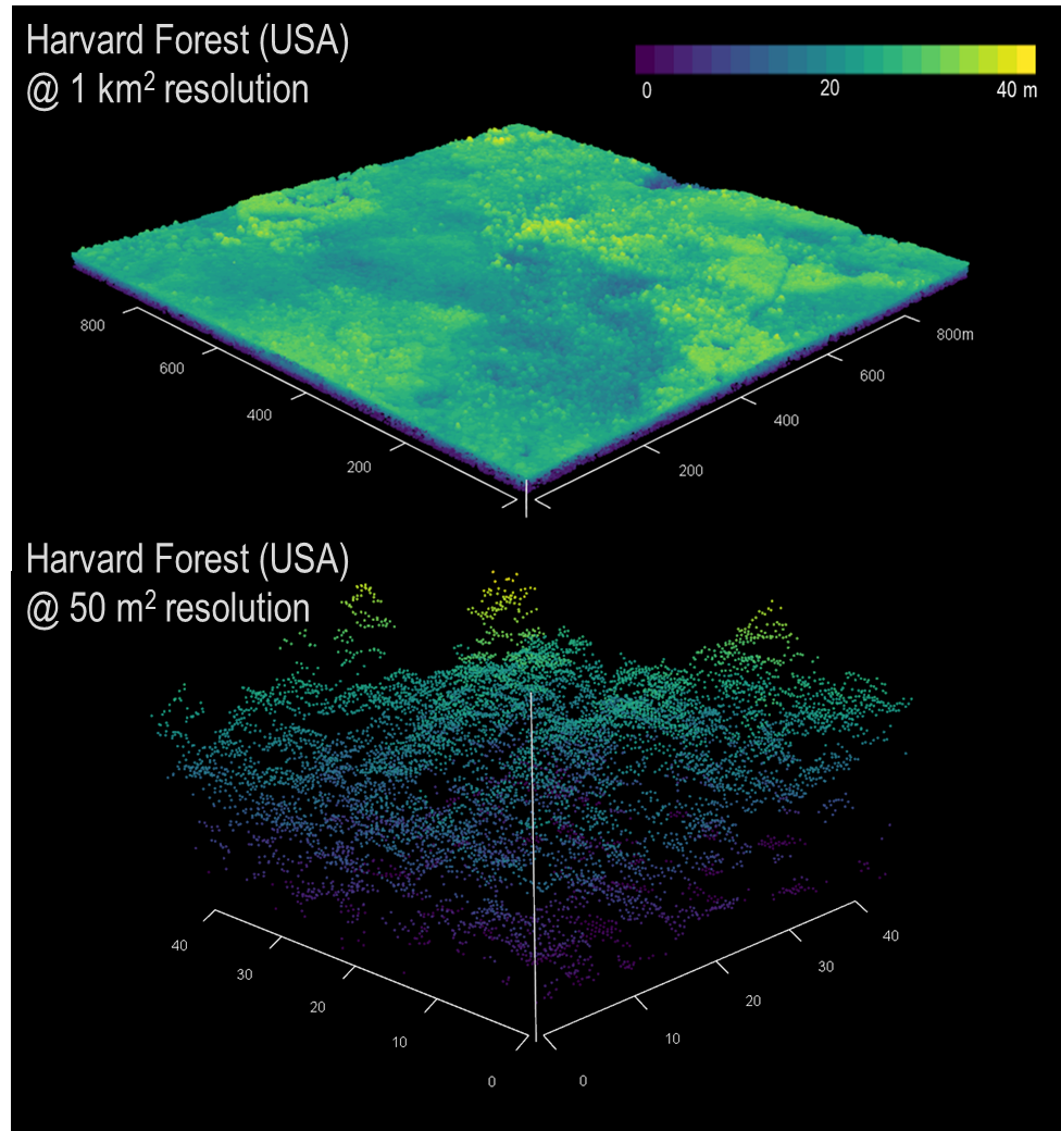
I have found myself increasingly curious about how forest structure, as inferred using LiDAR, scales. More plainly, let’s think about forest height. LiDAR is different from many other forms of remote sensing in that it has no native scale. The raw data are in the form of point clouds, individual estimates of height or distance at discrete points.

Compare this to satellite imagery (e.g., Landsat), which comes in the form of gridded, uniformly sized pixels. Landsat imagery is typically in the form of a raster of data, 1 km² in area with each pixel having a native resolution of 30 m—each pixel is one 30 x 30 m datum.

LiDAR point clouds often contain millions of points, each with an x, y, z value. X and y being the position on the ground and the z being the position above that x, y point. So already, we are adding another dimension. For each square meter on the ground, there can be anywhere from 2-3 points to as many as 12-15. While we focus on aerial LiDAR, which is collected from aircraft, LiDAR can also be collected from unoccupied aerial vehicles (UAV), ground-based scanners (terrestrial LiDAR or TLS), or from spaceborne satellites (e.g., GEDI, ICESat-2).

Challenges using LiDAR

In that raw form, LiDAR data are somewhat intimidating, necessitating the need to simplify to a more useful format. The most used data produced by LiDAR are canopy height models (CHMs). These, like Landsat data, are raster tiles of forest height. But herein lies the crux of the issue—at what resolution does one aggregate those LiDAR point returns to give a useful, representative height model?

The standard approach has not been to consider the LiDAR data directly. Rather, to use the resolution of interest for whatever problem is being addressed, or to aggregate LiDAR data to the same resolution of another data product that is being used in the analysis.

This rather arbitrary approach is one that has vexed me for a long time. How do we know what the “appropriate” resolution to use is? What can we do to apply a measure (no pun intended) of statistical rigor to how we aggregate lidar data for applications and research?

One possible solution borrowed from hydrology, and the one we explore in our manuscript, is Representative Elementary Area (REA). As Blöschl et al. (1995) wrote in Hydrological Processes,

“ [REA] . . . promises a spatial scale over which the process representations can remain simple and at which distributed catchment behaviour can be represented without the apparently undefinable complexity of local heterogeneity.”

We can think of REA as the spatial scale over which a process is measurable and statistically stable, thus allowing us to make more rigorous inferences.

Creating a standard scale

To apply the REA concept to LiDAR, we first needed to find a statistical way to identify the REA. We opted to use Changepoint Analysis, a statistical method that identifies when the probability distribution of a stochastic process or time series changes significantly.

With spatial data, approaches such as segmented regression are used.  In segmented regression, the range of an independent variable is broken into intervals with lines fit to those intervals. Then the slopes of those lines are tested to see if they differ significantly. If a difference is identified between slopes, that indicates a change in the relationship between the independent and dependent variable. Our analysis used the aggregation resolution as the independent variable. 

From segmented analysis we find the point at which those slopes differ, known as the “changepoint”. Using this changepoint with the associated confidence intervals, we can identify the REA for each LiDAR structural metric.

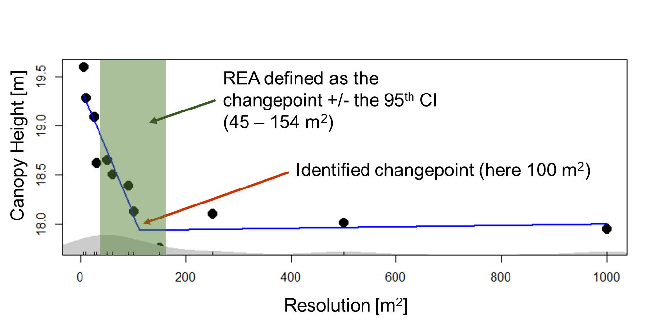
In the example above we are looking at forest canopy height. This was measured as the mean outer canopy height for Harvard Forest (USA) against the resolution—scale or grain size to which the canopy height values are aggregated. The changepoint, at 100 m, represents the average of the highest LiDAR return height for every 1 m² within a defined 100 m spatial grain (~1000 measurements).

The blue line shows the fitted segmented regression. In this example, spatial resolutions outside the upper and lower bounds of the REA (in green, above), are not representative of the forest stand. At lower spatial resolutions, we are seeing intra-canopy variation from individual trees. Above 154 m, we are seeing the influence of the landscape—changes in soils, landforms, or even climate.

If we were to perform an analysis at Harvard Forest to relate forest structure to some functional response (e.g., aboveground productivity, light use efficiency), aggregating height estimates to a spatial resolution between 45 and 154 m², based on our REA analysis, would provide a high degree of confidence that we are representing forest height sufficiently. This REA could be used with a high degree of confidence with any other temperate forest of similar age and composition.

Future of LiDAR

We also address other measures of forest structure, including canopy cover and higher-order derived metrics such as rugosity, foliar height diversity, and canopy relief ratio—metrics that describe the structural complexity of forests. We do find differences in the REA when we consider forest type (e.g., broadleaf, needleleaf).

The REA for some height metrics is lower for needleleaf forests, likely a function of those forests tending to be more even-aged, more uniform than the broadleaf forests used in this study. Also, the REA for canopy cover is higher in needleleaf forests, which could be a function of the individual architecture of leaves versus needles.

Additionally, applying methodologies and frameworks from other fields could greatly inform how we work with LiDAR not just in forests, but in all ecosystems. There is also an open question regarding the role of forest age, as we know that forest structure changes with age. Though again, this is system dependent as not all forests show a similar age-structural relationship.  

We hope that the REA concept will be useful to readers of MEE and to those working with LiDAR. The ability to characterize forest structure as an emergent property has many profound uses in ecological research and we are excited about the future.

Read the full article:

“Scale dependency of LiDAR-derived forest structural diversity”