Post provided by Anne Chao (National Tsing Hua University, Taiwan)

Shannon Entropy

Ludwig Boltzmann (1844-1906) introduced the modern formula for entropy in statistical mechanics in 1870s. Since its generalization by Claude E. Shannon in his pioneering 1948 paper A Mathematical Theory of Communication, this entropy became known as ‘Shannon entropy’.

Shannon entropy and its exponential have been extensively used to characterize uncertainty, diversity and information-related quantities in ecology, genetics, information theory, computer science and many other fields. Its mathematical expression is given in the figure below.

In the 1950s Shannon entropy was adopted by ecologists as a diversity measure. It’s interpreted as a measure of the uncertainty in the species identity of an individual randomly selected from a community. A higher degree of uncertainty means greater diversity in the community.

Unlike species richness which gives equal weight to all species, or the Gini-Simpson index that gives more weight to individuals of abundant species, Shannon entropy and its exponential (“the effective number of common species” or diversity of order one) are the only standard frequency-sensitive complexity measures that weigh species in proportion to their population abundances. To put it simply: it treats all individuals equally. This is the most natural weighing for many applications.

Estimating Entropy from Sampling Data

In practice, the true number of species and their relative abundances are almost always unknown, so the true value of Shannon entropy must be estimated from sampling data. The estimation of this seemingly simple function is surprisingly difficult, especially when there are undetected species in the sample. It’s been proven that an unbiased estimator for Shannon entropy doesn’t exist for samples of fixed sizes.

The observed entropy of a sample or the ‘plug in’ estimator, which uses a sample fraction in place of the relative abundance of species, underestimates the entropy’s true value. The magnitude of this negative bias can be substantial.

For incomplete samples, the main source of the bias comes from the undetected species, which are ignored in the plug-in estimator. An enormous number of methods/approaches have been proposed in various disciplines to obtain a reliable entropy estimator with less bias than that of the plug-in estimator. The diversity of the approaches reflects the wide range of applications and the importance of bias-reduction.

My Introduction to Alan Turing’s Statistical Work

Around 1975 (when I was a graduate in the Department of Statistics, University of Wisconsin-Madison) my advisor at the time, Bernard Harris, suggested that an “attractive and absorbing” (his original description) PhD thesis topic would be to develop an ‘optimal’ entropy estimator based on sampling data. He thought Alan Turing’s statistical work might prove to be useful and hoped that I could tackle this estimation problem.

However, at that time I didn’t even know who Alan Turing was! Although I started to read two background papers by I. J. Good (links below) about Turing’s statistical work, I couldn’t fully digest the material in the short time available. So, I didn’t work on the entropy estimation problem for my PhD thesis; instead, I derived some lower bounds for a variety of diversity measures. Ever since then, however, entropy estimation has fascinated me and has been in my mind/thoughts, and I regarded it as my ‘unfinished thesis’ topic.

The Building Blocks of My Entropy Estimators

According to I. J. Good (Turing’s statistical assistant during World War II), Turing never published his wartime statistical work, but permitted Good to publish it after the war. The two influential papers by Good (1953) and Good and Toulmin (1956) presented Turing’s wartime statistical work related to his famous cryptanalysis to crack German ciphers. After graduation, I read these two papers many times and searched for more literature. It took me a long time to fully understand these two papers especially Turing’s statistical approach to estimating the true frequencies of rare code elements (including still-undetected code elements), based on frequencies in intercepted ‘samples’ of code.

The frequency formula is now referred to as the Good-Turing frequency formula. Turing and Good discovered a surprisingly simple and remarkably effective formula that is contrary to most people’s intuition. The formula proved to be very useful in my development of entropy estimators.

One important idea derived from the Good-Turing frequency formula is the concept of ‘sample coverage’. Sample coverage is an objective measure of the degree of completeness of the intercepted ‘samples’ of code elements. The ‘sample coverage’ of a sample quantifies the proportion of the total individuals in the assemblage that belong to sampled species. Therefore, the ‘coverage deficit’ (the complement to sample coverage) is the probability of discovering new species, i.e. the probability that a new, previously-unsampled species would be found if the sample were enlarged by one individual. Good and Turing showed that for a given sample, the sample coverage and its deficit can be accurately estimated from the sample data itself. Their estimator of coverage deficit is simply the proportion of singletons (in this case species with only one individual) in the observed sample. This concept and its estimator play essential roles in inferring entropy.

A Novel Entropy Estimator

A species accumulation curve (SAC) shows the cumulative number of species as a function of sample size. In the figure below we see the expected curve when individuals are sequentially selected from a community with a given number of species, with relative abundances.

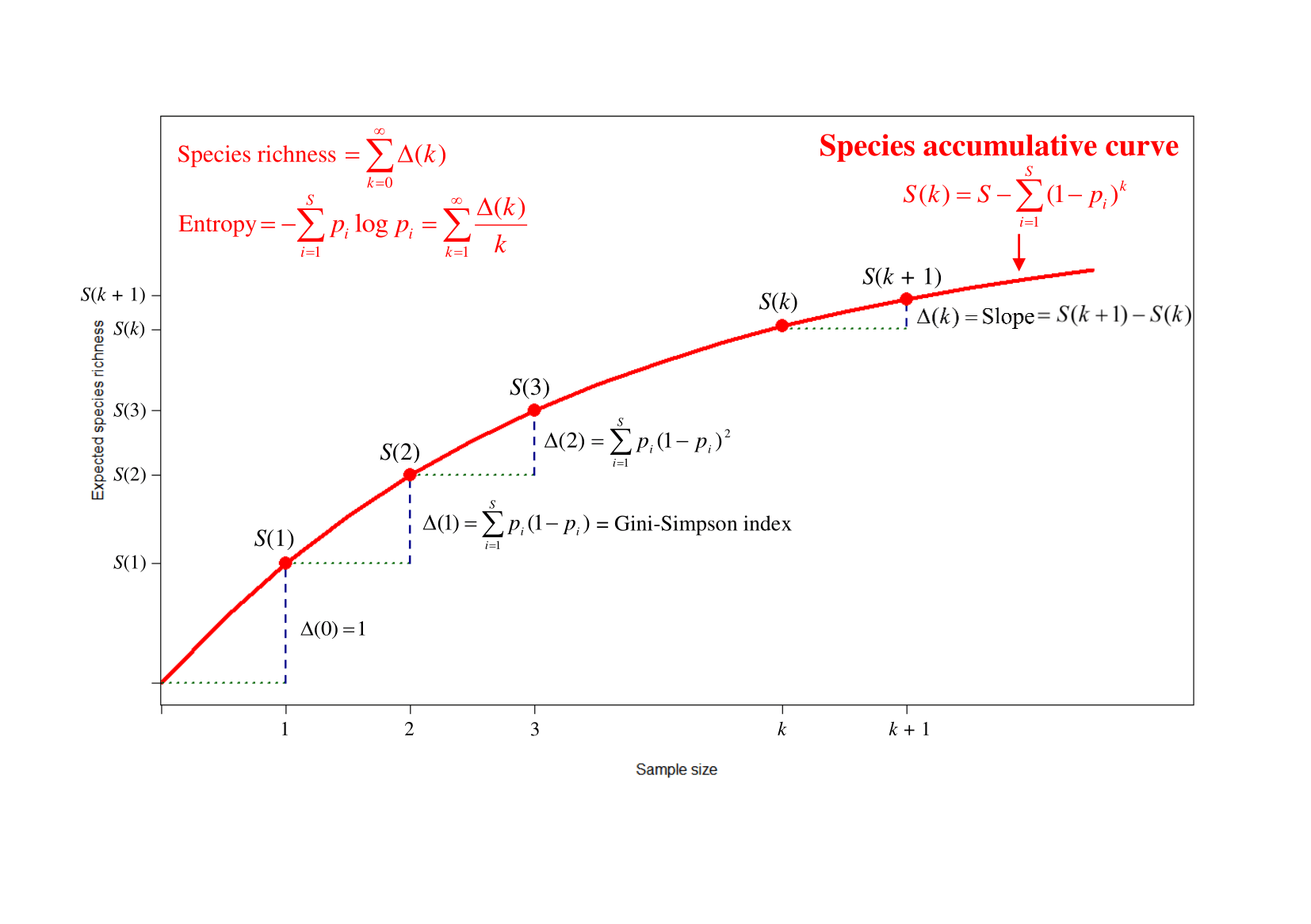
The first breakthrough in my search for an estimator of Shannon entropy was the realization that entropy can be expressed as a simple function of the successive slopes of the SAC. The curve’s successive slopes show the rates at which new species are detected in the sampling process. I had found a novel way to estimate entropy via discovery rates of new species in a SAC and these rates or slopes are exactly Turing’s coverage deficits for varying sample sizes!

The statistical problem was then to estimate the expected slopes or coverage deficits for any hypothetical sample size. Good and Turing’s approach provided the coverage deficit estimator for the expected slope of the sample that has been taken. All of the expected slopes for smaller sample sizes can be estimated without bias from statistical inference theory. However, there is no unbiased estimator for the expected slopes for sample sizes greater than the sample taken. These slopes are usually dominated by rare undetected species whose effect on entropy cannot be ignored. So, the burden of entropy estimation is shifted onto the estimation of the expected slopes for sizes greater than our sample.

The second break-through step to solve this problem was also attributed to the wisdom of Turing and Good, who showed that the number of singletons carry much information about the number of undetected rare species. I slightly modified their idea to use both singletons and doubletons to estimate the hard-to-estimate slopes by my modified Good-Turing frequency formula.

With the collaboration of Lou Jost and the simulation/programming work of Y.T. Wang, we published in 2013 the novel entropy estimator based on the derived slope estimators. Our extensive simulations from theoretical models and real surveys generally showed that the new estimator outperformed all the existing estimators. It took me over 35 years to derive the optimal estimator for my ‘unfinished thesis’, so I have been calling it my entropy ‘pearl’. (The novel entropy estimator along with other related estimators can be calculated online.)

Extending the Estimator to a Diversity Profile

The figure above also reveals that species richness can be expressed as the sum of all slopes, and the Gini-Simpson index is simply the slope at initial size 1. Moreover, diversities (Hill numbers) and entropies (Rényi entropies and Tsallis entropies) of any order q (the parameter which determines the measures’ emphasis on rare or common species) can all be expressed as functions of successive slopes of a species accumulation curve. Rather than selecting one or a few measures to describe the diversity of a community, we can convey the complete story by presenting a continuous profile: a plot of diversity or entropy as a function of q ≥ 0.

This “diversity profile” makes it easy to visually compare the compositional complexities of multiple communities. Based on sampling data, Lou Jost and I applied the same slope estimators as those used in estimating Shannon entropy to obtain an accurate and robust estimator for the true diversity profile from sample data. This estimated profile conveys all information about the species relative abundance distribution. Also, the profile approach can be extended to phylogenetic diversity and functional diversity.

Doing Research is like Carving Jade

I am sorry that Bernard Harris didn’t get to see the entropy ‘pearl’ that I obtained around July 2011 (and published in 2013). Unfortunately he passed away in January 2011. As the old saying goes: “doing research is like carving jade, we are never satisfied with what we have until it is perfect”. This is also my advice to anyone starting their career in academia. The topic of entropy estimation has attracted and absorbed me for more than 35 years, and hopefully the novel estimator did yield an ‘optimal’ solution, if it’s still not perfect.