Post provided by Oliver Metcalf

Acoustic indices are increasingly being used when analysing soundscapes to gain information on biodiversity. However, inconsistent results and lack of consensus on best practices has hampered their application in conservation and land‐use management contexts. In this post, Oliver Metcalf talks about his Methods in Ecology and Evolution article ‘Acoustic indices perform better when applied at ecologically meaningful time and frequency scales’, where he highlights the need to  calculate acoustic indices at ecologically appropriate time and frequency bins to reduce signal masking effects.

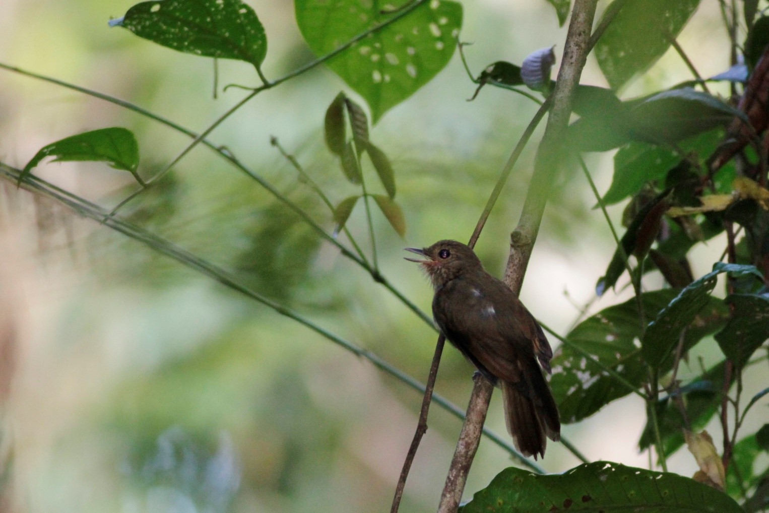
Monitoring biodiversity in one of the most species rich landscapes in the world is surprisingly hard, but listening to the soundscape can help. In 2017 I started my PhD at Manchester Metropolitan University (MMU) with the brief of using the latest advances in ecoacoustics to monitor change in community composition across variably-disturbed Amazonian rainforests in the Santarém region of Brazil with the Sustainable Amazon Network (RAS). The RAS network uses a range of ecological and social science methods to understand and mitigate the impact of forest disturbance and degradation across human-modified tropical forest landscapes, and I was keen to see what I could add to this already impressive body of work with the application of some cutting edge technology.

As I got to grips with the promises of artificial intelligence, I read voraciously about the potential to use the latest statistical toolkits to automatically identify animals from their vocalisations. Two things became abundantly clear; any attempt at using automated classification would require stacks of manually labelled training data, and the appeal of whole-soundscape approaches like acoustic indices that didn’t require species identification and therefore removed the heavy-lifting of manual labelling training data.

Nevertheless, for the time being I was sold on automated classification, and set about the mammoth task of labelling thousands of pieces of training data. The first thing that struck me was how beautiful spectrograms can be, with repeated patterns, variations, swirls and occasional violent slashes – almost like modern art. Second was just how variable they are, no two spectrograms look the same, reflecting the changing nature of rainforest soundscapes.

As I labelled more data, patterns began to emerge. By this stage, I was focussing on nocturnal species, and it became clear that nocturnal birds in the region I was working on only vocalized below 4 kHz, above that there was just too much insect noise for the birds to compete with – the species had, to an extent, taxonomically compartmentalized themselves in acoustic space. I also began to play a game with myself, could I guess the time of night that spectrograms came from without looking at the metadata, and I found that more often than not, by a looking at a few minutes of data I was normally correct. The tell-tale signs seemed to be the intensity of insect noise between 4-8 kHz (that I’d come to know as the blackout curtain, as insect sound was usually so intense, it resembled an indistinguishable black band), the amount of streaking from katydids and other insects above 10 kHz, and the number of birds calling below 4 kHz. Even without knowing many of the species involved, the spectrograms began to segment themselves in to almost definable groupings by time and frequency, with distinctive patterns at different time and frequencies.

By late 2018, as I think is normal for many PhD students, my attention had begun to drift from focussing on the single goal of automated classification. Thankfully my excellent supervisory team Alexander Lees, Stuart Marsden (MMU), and Jos Barlow (Lancaster University) reminded me of the alternative approaches discussed at the outset, and I began to look again at the potential applications of acoustic indices. This coincided with the BES Tropical Ecology conference in Edinburgh, and some excellent discussion and presentations there persuaded me of the utility of this approach.  

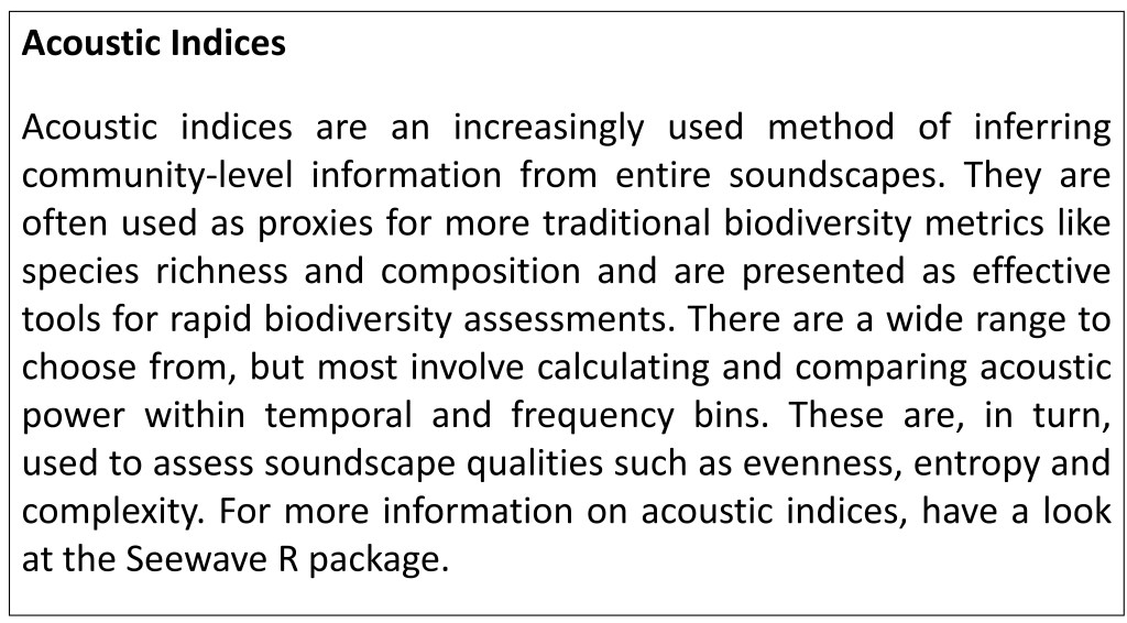
Acoustic Index Sensitivity

Investigating further, I was surprised by how broadly researchers have applied indices to acoustic data, typically aggregating index values across long periods of time and across the entire frequency spectrum. There were some excellent studies that seemed to show that a combination of indices could be used to characterise different habitats or disturbance regimes but weren’t always completely accurate when comparing very similar habitats, or required computation of many different indices. I hypothesized that as different taxonomic groups were likely to respond differently to differing landscapes or disturbance, calculating indices across broad domains was likely to mask such subtleties. However, it seemed likely that by measuring the indices at narrower frequency ranges and at smaller timescales, we could capture that complexity. And that by capturing that complexity, acoustic indices would be better at characterising different locations. My co-authors and I set out to find out if this was the case, using two of the most commonly used acoustic indices – the Acoustic Complexity Index and the Biodiversity Index.

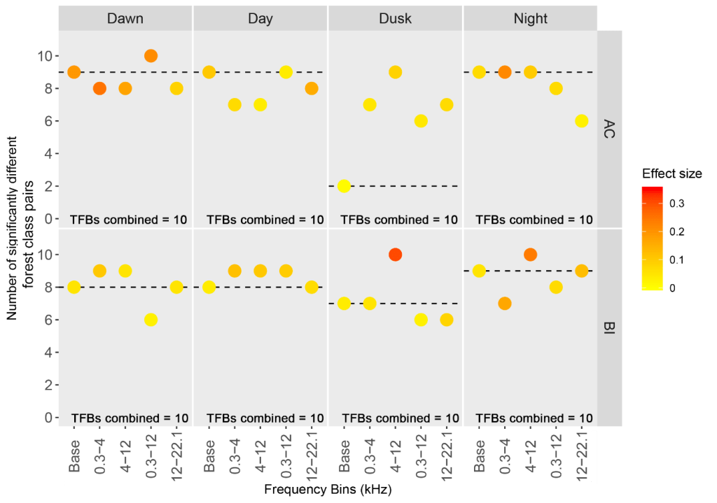
The data was partitioned temporally into dawn, dusk, day and night, and split into frequency bins reflective of the patterns I had observed whilst labelling data, with these observations supported by previous research on acoustic niches.

We used the indices values from the different time-frequency bins and tested for significant differences from the other forest classes. Unsurprisingly the broadest bins worked well, often as good or better than any one of the narrower bins at differentiating between forest classes. This was expected, after all, you would expect primary forest to have a different soundscape to, for example secondary forest, across all or most frequency bins. However, the broadest frequency bins didn’t contain significant differences between all of the forest classes. There was always one, two, or more of the most similar forest classes that weren’t significantly different. When we used all of the narrower bins, we did find significant differences between all of the classes.

We argue that this is because using broad ranges for measuring indices don’t fully capture the complexity of taxonomic response to different habitats. For instance, cicadas that stridulate at 5-8 kHz in the middle of the day might increase in forests that let in more light, but bird species that feed on the ground and call at 0.5-2 kHz at night might decrease. Trying to characterise soundscapes in a single measure masks these responses. Instead, it’s better to use a range of (ecologically meaningful) time and frequency bins. We saw the scale of the improvement when we used our indices data as training variables in a Random Forest to predict forest class – with the broadest frequency bands accurately predicting forest class just 62.1% of the time when differentiating between all five forest classes, and the range of narrower bins being 88.2% accurate.

Acoustic Index fidelity

Acoustic indices are also employed to measure the diversity of particular groups, for instance as a proxy for bird diversity. But given the acoustic masking across taxonomic groups, we wanted to know how much indices measured broadly responded to general acoustic diversity, rather than the diversity of the taxonomic group in question. We correlated species richness data obtained through manually identifying bird species at dawn and at night in our acoustic data with the acoustic index scores. Again, here we found evidence of acoustic masking. The acoustic index values from the broadest bins showed either weaker correlations or sometimes even inverse correlations to the narrow frequency bins that contained most bird song. In other words, measuring acoustic indices at broad time and frequency spans led to indices having lower fidelity to the diversity they were intended to measure.

Summary

We believe that using acoustic indices at narrower time and frequency bins can greatly improve the efficacy of acoustic indices, both in characterising landscapes and as a proxy for biodiversity. To some, the requirement of a priori ecological knowledge to inform the boundaries of these bins may seem an onerous requirement. However, we believe that a relatively short amount of time reviewing acoustic recordings and the application of some ecological common sense can result in some big improvements in the functioning of acoustic indices, as was the case for us!

We only used two acoustic indices, Acoustic Complexity and the Biodiversity Index, but many more exist. For more on the impact of acoustic masking on a range of indices, take a look at Ross et al., (2020), published almost simultaneously to our own work, and providing some very interesting complimentary findings.

To read the full Methods in Ecology and Evolution article, ‘Acoustic indices perform better when applied at ecologically meaningful time and frequency scales’, visit the journal website here.