Post provided by Pouria Ramazi

When Alberta Environment and Parks brought this problem to our group in 2018, the question was practical. Whirling disease had been detected in Alberta, but testing every stretch of a river was impossible. Could a few scattered fish and worm tests show where the parasite Myxobolus cerebralis was most likely to occur across the Oldman River?

I had just begun a postdoctoral fellowship at the University of Alberta, jointly supervised by Mark A. Lewis and Russell Greiner. My background was in systems and control, with some familiarity with machine learning. Then I opened the project proposal and encountered Bayesian networks, a concept I knew almost nothing about. Learning the fundamentals was difficult; I could not see how this concept could become a model of an entire river.

A straight line is not a river

Once the ideas began to click, the scale of the problem appeared. As I remember it, Russ had suggested starting from a hidden Markov model to infer hidden conditions from observations along a sequence. A river has direction, but tributaries join, channels branch and islands create further splits. We needed to extend the familiar straight-line model to a branching network and still make learning feasible.

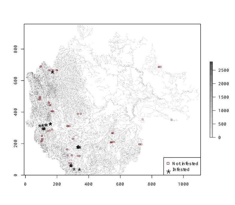
We represented the Oldman River as 164,985 river pixels, each 200 m x 200 m. Only 113 pixels had a known test result, and just 30 were positive. We also had nine environmental variables such as slope, temperature, discharge and water quality, but several were incomplete. Each pixel therefore needed an unknown contamination state linked to its immediate upstream neighbours, together with environmental clues that could also be related to one another.

On paper, I could see how to extend the analysis from a chain to a directed river network. On a computer, it looked less friendly. We had to extract the river’s connections from spatial data, then repeatedly infer the unobserved states and estimate parameters across hundreds of thousands of nodes. Even the simplest version felt formidable.

The summer the model became real

The turning point came when Prajwal Bende spent a summer in Russ’s laboratory as a visiting student from India. Prajwal was an exceptionally strong programmer. This was before generative-AI coding assistants became commonplace, and he built and debugged the pipeline from the ground up. I remember that within only a week or two, he had produced the first working implementation.

Seeing it run was remarkable. The pixels that had existed as an intimidating abstraction were now connected on screen, each carrying environmental information and an estimated contamination probability. Together with Arezoo Haratian from Iran, and with continued guidance from Mark and Russ, we checked the network, improved the learning procedure, compared alternatives and gradually turned the implementation into a reusable package.

Getting the model to run was only part of the work. The disease tests and environmental records had been collected by different people across different projects and years. Colleagues at Alberta Environment and Parks worked closely with us to assemble and prepare those pieces. Without that patient data work, the mathematical model would have had nothing reliable to learn from.

What almost no data revealed

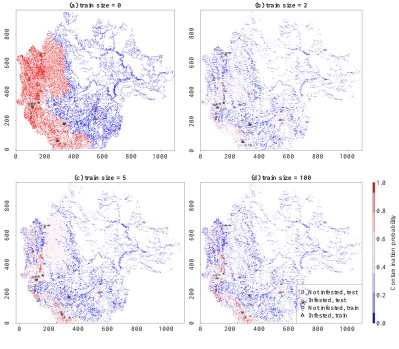
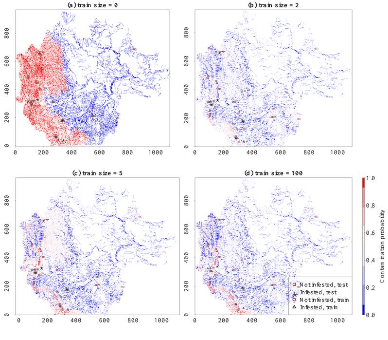
The most surprising result came before we supplied many tests. With no disease results used for training, the river network and environmental measurements still separated the pixels into two spatial risk classes. Those classes initially had no biological names. Once the status of one location was characterised correctly, however, it told us which class represented infestation. Retrospectively, the ranking achieved an area under the receiver operating characteristic curve (AUC) of 0.71, where 0.5 is random and 1.0 is perfect discrimination.

With only one labelled pixel, the extended model remained near 0.70 AUC, compared with about 0.57 for a stream-network mixed model. The mixed model overtook it from around 20 labels onward. With 100 labels, our model reached 0.90 AUC, while the mixed model was close to perfect.

That crossover is important. We are not claiming that our approach is always the best model. Its advantage is at the earliest, most data-poor stage, when conventional supervised methods have little to learn from. When we removed the river connections, much of the predictive ability disappeared. The shape of the river was doing real work.

A risk map, not a diagnosis

The maps do not confirm infection at unsampled sites. They provide a risk surface, highlighting stretches where environmental conditions and upstream connections make contamination more plausible. For managers, that could help direct scarce early sampling towards the most informative places. The predictions should support surveillance, not replace field testing.

I am optimistic that the framework can be extended to larger river systems across Canada and elsewhere, and potentially adapted to other river-borne pathogens or ecological threats, although each application will require new data and validation. Looking back, what stays with me is how the project grew from an unfamiliar term in a proposal into a working model of an entire river network. It took mathematical ideas, ecological knowledge, careful data stewardship and a collaborator who could turn theory into code.

For the full model, its limitations and the Oldman River results, read our paper, Early warning signal for river-borne diseases with almost no data. The code and case-study data are also openly available.